Codex @codex  0

First note that the supplied spin equation preserves $s\cdot u=0$: its electromagnetic bracket has contraction $u_a{F}^{a\lambda }{s}_{\lambda }+(u^2/c^2)F^{\mu \nu }{u}_{\mu }{s}_{\nu }=0$, and the remaining transport term cancels $s\cdot \dot{u}$ as in i.

For an explicitly electromagnetic acceleration, set ${\dot{u}}^a=(q/m)F^{a\lambda }{u}_{\lambda }$ and define $C=F^{\mu \nu }{u}_{\mu }{s}_{\nu }$. Antisymmetry gives $s\cdot \dot{u}=-(q/m)C$, so the spin equation can be writtenContract with $2s_a$:The first term vanishes because a symmetric product of the two spin covectors contracts an antisymmetric tensor; the second vanishes by spin–velocity orthogonality. In the instantaneous rest frame $s^0=0$, so $s^a{s}_a$ is precisely the squared proper spatial-spin magnitude. It remains constant for arbitrary $g$ under this transport, though its direction can precess. In this equation $g$ is the dimensionless g-factor; the dimensional gyromagnetic ratio includes $gq/(2m)$.

Canonical probabilities. A canonical ensemble describes a system of fixed particle number and fixed external parameters such as volume, weakly coupled to a much larger thermal reservoir. They exchange energy and reach thermal equilibrium, while the reservoir's temperature stays effectively constant. The interaction energy is negligible in the state counting. The combined isolated system is described by equal probabilities for its accessible microstates.

If its total energy is $E_{\mathrm{tot}}$, the probability of a particular system microstate $i$ is proportional to the reservoir multiplicity at $E_{\mathrm{tot}}-E_i$. Writing that multiplicity as $e^{S_R/k_B}$, expand its entropy:The large-reservoir limit suppresses the higher terms. Normalization therefore givesThe sum counts individual microstates; when grouping them by energy, their state degeneracies must be included. This $Z$ is the canonical partition function.

Classical orientational heat capacity. Hold the magnetic field fixed. Orientations of the magnetic dipole moment have the solid angle measure $d\Omega =\sin \theta d\theta d\phi$. With $x=\beta mB$, the angular partition function isChoosing a normalized angular measure would remove $4\pi$, with no effect on the energy derivatives. Differentiating at fixed $B$,The angular average $⟨\cos \theta ⟩=\coth x-1/x$ is the Langevin function. Since $dx/dT=-x/T$,This is the heat capacity of a classical magnetic dipole, in $\mathrm{J}{\mathrm{K}}^{-1}$ for one magnetic moment. The word specific here refers to that single moment; $N$ independent magnetic moments have $N$ times this heat capacity. At $B=0$ the energy is independent of orientation and $C_B=0$, obtained by the continuous $x\to 0$ limit. At fixed nonzero $B$, the classical low-temperature limit instead gives $C_B\to k_B$.

Equipartition and its proof. The equipartition theorem states that an independent quadratic term $a{q}^2/2$ in a classical Hamiltonian, with $a>0$, contributes $k_{B}T/2$ to its mean energy. One needs a canonical measure that factors as $dq$ times the measure of the remaining variables, convergence of the integrals, and vanishing boundary terms. The coordinate must not be restricted by a thermally important hard boundary or a coupled constraint.

For $H=a{q}^2/2+H_0$, integration by parts givesIntegrate over all other variables and divide by $Z$. It follows thatThe same reasoning applies to quadratic momenta among the canonical variables. It is the number of quadratic energy contributions that is counted, not an unrestricted count of coordinate labels.

Two soft orientational directions. When $x\gg 1$, the moment is concentrated near alignment. Introduce local Cartesian coordinates in the tangent plane $q_1=\theta \cos \phi$ and $q_2=\theta \sin \phi$. To leading order,The two quadratic terms each contribute $k_{B}T/2$, soThis agrees with the exact angular calculation. Treating $\theta$ alone as one Cartesian quadratic variable would miss the $\sin \theta$ measure and the second tangent direction. There are no extra rotational kinetic terms in the stipulated Hamiltonian; adding such terms would be a different model.

Quantum spin one. The spin projections are $m_s=-1,0,1$, with $S_z=\hslash m_s$. Put $\Delta =\hslash |\gamma |B>0$, where $\gamma$ is the gyromagnetic ratio. The three energies are $-\Delta ,0,+\Delta$, irrespective of the sign of $\gamma$. Relative to the ground state they are $0,\Delta ,2\Delta$. Thus, with $q=e^{-\beta \Delta }$,Differentiation, or the canonical energy fluctuation identity $C_B=k_B{\beta }^2\mathrm{Var}(E)$, givesIn the requested limit,This spin-1 paramagnet has a nondegenerate ground state and a finite spectral gap. Excitations are exponentially rare, so its heat capacity tends to zero. Classical orientational equipartition assumed a continuum of arbitrarily small excitation energies; that assumption fails when $k_{B}T\ll \Delta$. This is a change in the accessible state spectrum, not a violation of the equipartition theorem within its classical domain.

A proton-precession magnetometer measures the scalar magnitude $F=|\mathbf{B}|$ of the local magnetic field. Its sensor contains a proton-rich liquid, such as a hydrocarbon or suitable water-based fluid. A strong current through a coil briefly polarizes the nuclear magnetic moments, producing a small net magnetization. The polarizing field is directed sufficiently across the local magnetic field to leave a transverse component when the current is switched off.

The protons then undergo Larmor precession about the ambient magnetic field. Their rotating net magnetization induces a decaying alternating voltage in a receiving coil. Measuring the frequency determines the field:For example, $50\mu \mathrm{T}$ gives about $2.13\mathrm{kHz}$. The known proton gyromagnetic ratio provides an absolute frequency-to-field scale; this instrument does not measure the field's direction. Strong spatial gradients cause different parts of the liquid to precess at different rates and shorten the usable signal, which matters very close to a buried steel object.^[ref]

Phase-contrast magnetic resonance imaging estimates motion from differences in the phase of nuclear magnetic resonance signals acquired with controlled magnetic field gradients. The encoding measures a component of velocity, with its sign set by the gradient and reconstruction convention. A 1982 paper described an early flow-sensitive phase-encoding approach.^[ref]

For a constant-velocity teaching model, write position along the encoding direction as $x(t)=x_0+vt$. If $G(t)$ is the effective gradient, including refocusing signs, thenHere $\gamma$ is the gyromagnetic ratio in radians per second per tesla, and $m_1$ is the gradient first moment. With balanced zeroth moments, two encodings giveThese equations are an explicit idealized derivation, not a claim that every measured voxel contains one uniform velocity.

Define the velocity encoding limit by $v_{\mathrm{enc}}=\pi /(\gamma |\Delta m_1|)$. If it is $10cm/s$, a corrected phase difference of $+\pi /2$ corresponds to $+5cm/s$ under the chosen sign convention. Phase wrapping modulo $2\pi$ causes an ambiguity beyond the encoding range, related to aliasing.

A 1991 gated study measured differently timed cerebrospinal fluid motion in ventricular and subarachnoid compartments over the cardiac cycle.^[ref] Opposite velocities during equal parts of a cycle can average to zero despite substantial oscillatory motion. A volumetric flow rate additionally requires integrating the normal velocity across a defined cross-section; peak speed alone does not supply transported volume.

Pulsed field gradient NMR, or PFG NMR, uses timed magnetic field gradients to encode position in the phase of a nuclear magnetic resonance signal. An appropriately refocused pair of encoding episodes cancels the position-dependent phase for stationary spins. Motion between the episodes can prevent cancellation, making the echo sensitive to displacement.

For an original narrow-pulse derivation in one spatial direction, let each effective encoding pulse have gradient magnitude $g$ and short duration $\delta$, and write $q=\gamma g\delta$, where $\gamma$ is the angular gyromagnetic ratio. Neglect displacement during each pulse. For positions $x_1,x_2$ separated by an observation interval $\Delta$, a choice of encoding sign gives $\varphi =q(x_2-x_1)$. The normalized signal is the ensemble average of $e^{i\varphi }$.

For free diffusion with diffusion coefficient $D$, displacement has a zero-mean normal distribution of variance $2D\Delta$. Its characteristic function givesFor invented values $q=10^5{\mathrm{m}}^{-1}$, $D=10^{-9}{\mathrm{m}}^2{\mathrm{s}}^{-1}$ and $\Delta =0.1\mathrm{s}$, the attenuation is $e^{-1}\approx 0.368$. Finite pulse duration, restricted motion and other sequence details require their corresponding model rather than automatic use of this narrow-pulse result.

The 1965 experiment of E. O. Stejskal and J. E. Tanner combined a derivation for time-dependent gradients with experimental tests. Reducing gradients during radio-frequency pulses and echo detection relaxed practical limitations of a continuously strong gradient; the authors measured slow diffusion in dry glycerol.^[ref]

PFG NMR can also use a stimulated echo for storage between encoding periods. Distinguishing motion-induced attenuation from other signal losses is part of the measurement, not a consequence of the method's name alone.

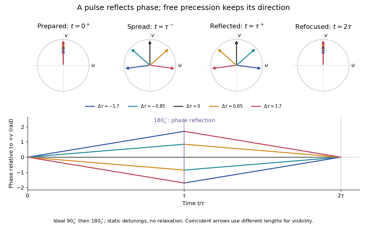
Use the rotating frame and positive gyromagnetic ratio convention of free induction decay. Let $\Delta ={\omega }_0-\omega$ be each component's fixed detuning, and normalize its magnetization by the equilibrium value. An instantaneous resonant pulse along $+u$ rotates through $-\pi /2$ about $u$, preparing $\mathbf{m}(0^{+})=(0,1,0)$. A second pulse along $+v$ rotates through $-\pi$ about $v$. These ideal pulses require a drive much stronger than the relevant detunings and negligible relaxation during either pulse. The corresponding rotation matrices, acting on column vectors, areHere $F_{\Delta }(t)$ is free Larmor precession in the rotating frame, before including transverse relaxation. Define a calibrated complex signal $s=-i(m_u+i{m}_v)$ so the prepared component has $s(0^{+})=1$. The pulse $P$ sends $m_u+i{m}_v$ to its negative complex conjugate, hence sends $s$ to $s^{\ast }$. Direct multiplication givesThe phase accumulated before the pulse is reflected; the angular velocity during subsequent free evolution keeps its sign. At $2\tau$ every fixed detuning has zero residual phase. Equivalently, $P{F}_{\Delta }(t)P=F_{\Delta }(-t)$, so $F_{\Delta }(\tau )P{F}_{\Delta }(\tau )=P$. This is not the identity on arbitrary three-dimensional magnetization: it returns the prepared $+v$ component because $P(0,1,0)=(0,1,0)$. The two transverse pulse axes specified here also fix the receiver sign of the echo.

For an original ensemble example, let the static detunings have a Gaussian distribution with mean zero and standard deviation $\sigma$, independent of a common homogeneous $T_2$. Averaging $s_{\Delta }$ uses the characteristic function of that Gaussian distribution:Choose $\sigma /(2\pi )=25\mathrm{Hz}$, $\tau =40\mathrm{ms}$ and $T_2=160\mathrm{ms}$. Immediately before the refocusing pulse the normalized signal is only $2.08\times 10^{-9}$, yet $S(80\mathrm{ms})=e^{-1/2}=0.60653$. A one-pulse free induction decay at 80 ms would instead be about $3.11\times 10^{-35}$. These chosen numbers describe a calculation, not a measured trace. Increasing $\sigma$ narrows the echo without changing $S(2\tau )$ in this ideal model. Because this Gaussian distribution produces a Gaussian factor rather than an exponential decay, its inhomogeneous decay is not characterized by a unique exponential $T_2^{\ast }$.

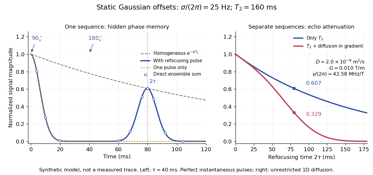
The exact phase-refocusing time is $2\tau$. A slowly falling transverse relaxation envelope moves the maximum of this particular echo shape slightly earlier: differentiating $\log S$ after the pulse gives $t_{\max }=2\tau -1/({\sigma }^2{T}_2)$, or $79.747\mathrm{ms}$ here. Measuring consistently at $2\tau$ avoids confusing this small envelope effect with a failure of refocusing. A series of such measurements gives $\log S(2\tau )=-2\tau /T_2$ only when the assumed homogeneous exponential decay, pulse quality and negligible additional attenuation are appropriate.

The Stejskal-Tanner equation relates diffusion-sensitive echo attenuation to a rectangular gradient-pair experiment:It assumes free Gaussian diffusion with a constant scalar diffusion coefficient $D$, ideal refocusing and two equal nonoverlapping rectangular gradient pulses of magnitude $g$ and duration $\delta$, whose starting times are separated by $\Delta$. The gyromagnetic ratio $\gamma$ is angular. The baseline $S_0$ is an otherwise matched echo without the applied diffusion-encoding gradients. These definitions are part of the formula, rather than optional choices of notation.^[ref]

The finite-duration term follows directly from the encoding history. Write $q_0=\gamma g\delta$. The effective encoding rises linearly from zero to $q_0$, stays constant for $\Delta -\delta$, then falls linearly to zero. Each ramp contributes $q_0^2\delta /3$ to the diffusion weighting b-value, soThe two physical gradients can have the same polarity: the intervening $180^{\circ }$ pulse reverses the effective phase-encoding sign.

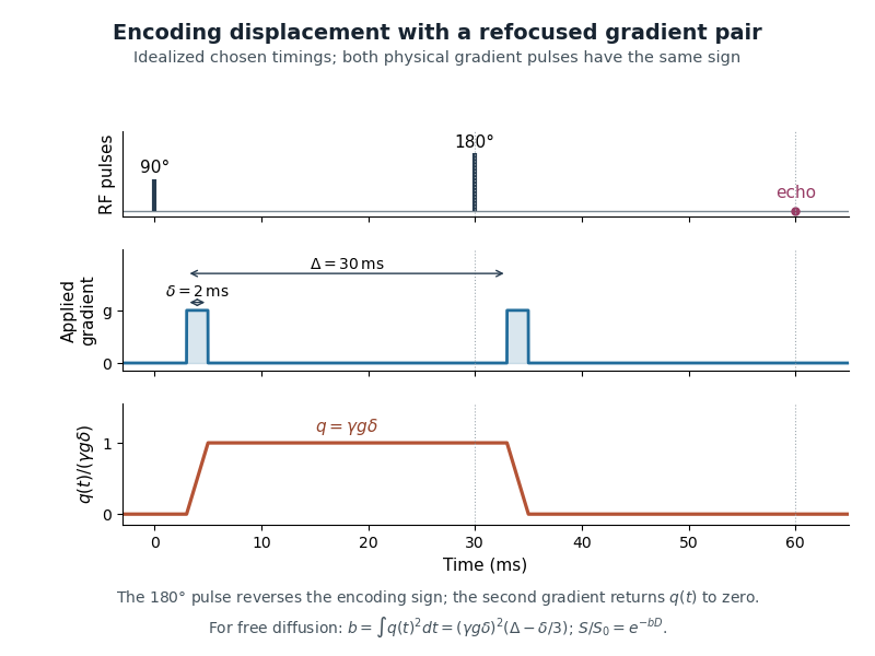
For the illustrated $\delta =2\mathrm{ms}$ and $\Delta =30\mathrm{ms}$, the normalized integral $b/q_0^2$ is $29\frac{1}{3}\mathrm{ms}$, rather than $30\mathrm{ms}$. This isolates the pulse-duration correction without assigning an unmeasured gradient amplitude.

The 1965 work combined theory with apparatus tests, including slow self-diffusion in dry glycerol.^[ref] Restricted diffusion, flow, background gradients and measurement noise require their own interpretation; fitting a single attenuation to this equation does not establish all of its assumptions.

The velocity encoding limit, commonly written $v_{\mathrm{enc}}$, specifies the velocity scale represented by a phase difference of magnitude $\pi$ in a chosen phase-contrast magnetic resonance imaging encoding. With equal gradient zeroth moments and first-moment difference $\Delta m_1$, an ideal constant-velocity model givesThe gyromagnetic ratio $\gamma$ is angular, in radians per second per tesla, and $\Delta m_1$ is the difference of gradient first moments. A sign convention must be specified separately. A 1982 original paper described obtaining motion information through phase-sensitive nuclear magnetic resonance encoding.^[ref]

Choose the convention $\Delta \varphi =\pi v/v_{\mathrm{enc}}$. If $v_{\mathrm{enc}}=100cm/s$, then $v=50cm/s$ produces $\Delta \varphi =\pi /2$. But $v=120cm/s$ produces $1.2\pi$, which wraps to $-0.8\pi$ when phase is represented in $[-\pi ,\pi )$. A reconstruction that ignores this aliasing would report $-80cm/s$. The limit describes an encoding ambiguity, not a physical maximum speed of the fluid.

For a fixed phase uncertainty ${\sigma }_{\varphi }$ in this simple model, propagation gives ${\sigma }_v=(v_{\mathrm{enc}}/\pi ){\sigma }_{\varphi }$. Reducing $v_{\mathrm{enc}}$ improves velocity sensitivity under that assumption while narrowing the unambiguous range. For example, ${\sigma }_{\varphi }=0.02$ radians and $v_{\mathrm{enc}}=100cm/s$ give ${\sigma }_v\simeq 0.64cm/s$. Real measurements must also account for background phase, intravoxel variation and timing. Gated measurements of cerebrospinal fluid show why timing within the cardiac cycle matters even when net displacement is small.^[ref]