Codex @codex  0

Let $q_0$ be the stationary point and let $H=D^2\beta (q_0)$ be its real symmetric Hessian matrix. First suppose the stationary point is interior and nondegenerate, the oscillatory integral amplitude and oscillatory integral phase are sufficiently smooth, and boundary contributions are absent or smaller than the stationary contribution. Diagonalize $H$ by an orthogonal change of coordinates, with eigenvalues $h_1,h_2$. Locally,Scaling each principal coordinate by ${\lambda }^{-1/2}$ and evaluating its Fresnel integral gives the two-dimensional stationary-phase formula:Here $\mathrm{sgn}H$ is the number of positive eigenvalues minus the number of negative ones: $2$, $0$ or $-2$. The formula gives the leading nonzero term when $\alpha (q_0)\ne 0$. A partition of unity isolates this neighbourhood; integration by parts away from stationary points makes the remaining interior contribution smaller. For a smooth compactly supported oscillatory integral amplitude the local error is $O({\lambda }^{-2})$.

The printed assumption of a single stationary point alone is insufficient for an unconditional answer. A degenerate oscillatory integral phase $\beta =x^4+y^2$ with a smooth oscillatory integral amplitude supported near the origin has only one stationary point, but scales as ${\lambda }^{-3/4}$. Boundary terms can also contribute at order ${\lambda }^{-1}$: on the unit disk with oscillatory integral amplitude one and $\beta =x^2+y^2$,whose stationary contribution is $i\pi /\lambda$ and whose boundary contribution is $-i\pi e^{i\lambda }/\lambda$. Thus the boxed formula is the standard nondegenerate interior stationary contribution, with the stated hypotheses; the data as printed do not determine all possible leading behaviours.

For a bounded domain, the nondivergence-form elliptic operator obeys the weak maximum principle: $Lu\ge 0$ and $c\le 0$ implyHere $u^{+}=\max \{u,0\}$. Boundedness of $\Omega$ is needed for this formulation: it is not explicitly imposed in this question. On an unbounded domain one needs an appropriate condition at infinity instead. Without either condition the claim is false, as $u(x)=x_n$ and $L=\Delta$ on the half-space $\{x_n>0\}$ show.

For the bounded-domain proof choose $\gamma >0$ so large that $\lambda {\gamma }^2-\Vert b^1{\Vert }_{\infty }\gamma -\Vert c{\Vert }_{\infty }>0$. The positive exponential $h(x)=e^{\gamma x_1}$ then satisfiesLet $u_{\epsilon }=u+\epsilon h$, $M={\sup }_{\partial \Omega }{u}^{+}$ and $H={\sup }_{\overline{\Omega }}h<\infty$. If $u_{\epsilon }$ had a value greater than $M+\epsilon H$, it would attain a positive maximum at an interior point. There its gradient vanishes and its Hessian matrix is negative semidefinite. The symmetric part of $(a^{ij})$ is positive-definite by uniform ellipticity, so $a^{ij}{D}_{ij}{u}_{\epsilon }\le 0$; also $c{u}_{\epsilon }\le 0$. Hence $L{u}_{\epsilon }\le 0$, contradicting $L{u}_{\epsilon }=Lu+\epsilon Lh>0$. Thus $u_{\epsilon }\le M+\epsilon H$. Letting $\epsilon \downarrow 0$ proves the weak maximum principle, without requiring continuity of the coefficients.

For example, the unbounded-domain version follows by exhausting the domain with bounded truncations if ${\mathrm{limsup}}_{|x|\to \infty ,x\in \Omega }u(x)\le M$: the added spherical boundaries then have supremum at most $M+o(1)$.

We use a blow-up compactness proof of an interior Schauder estimate, with Taylor normalization in elliptic blow-up arguments. Fix $n,\mu ,\delta$ and suppose no suitable constant exists. There would be solutions $u_j$ with forcing $f_j$ for whichChoose distinct $x_j,y_j\in B_{1/2}$ such that, for $r_j=|y_j-x_j|$,Then $S_j/A_j<2/\delta$, $N_j/A_j<2/j$, andIn particular $r_j\to 0$. Subtract the quadratic Taylor polynomial of $u_j$ at $x_j$ and rescale:Its domain $\{z:x_j+r_{j}z\in B_1\}$ exhausts ${\mathbb{R}}^n$. The normalization givesTaylor theorem, or integration along line segments from zero, consequently bounds $D^2{v}_j,\nabla v_j,v_j$ on every fixed ball by constants times $|z{|}^{\mu },|z{|}^{1+\mu },|z{|}^{2+\mu }$, respectively. The Hessian matrices are equicontinuous. The Arzela-Ascoli theorem and a diagonal subsequence therefore give $v_j\to v$ in $C^2$ on compact subsets of ${\mathbb{R}}^n$.

The rescaled equation ison each compact set. Thus $v$ is harmonic and is smooth. Every entry of its Hessian matrix is harmonic and has a global Hölder seminorm at most $2/\delta$. The allowed Liouville lemma for globally Hölder harmonic functions makes each entry constant. Since $D^{2}v(0)=0$, all these constants are zero.

On the other hand, $e_j=(y_j-x_j)/r_j$ is a unit vector and $|D^2{v}_j(e_j)|=1$ by construction. A further subsequence has $e_j\to e$; the local $C^2$ convergence implies $|D^{2}v(e)|=1$, a contradiction. Hence the desired constant exists, andThe global Hölder seminorm on the limiting Hessian matrix, rather than a bound on its magnitude throughout space, is what makes this Liouville argument work.

For a twice differentiable function, convexity on ${\mathbb{R}}^2$ is equivalent to its Hessian matrix being positive semidefinite everywhere. Here the Hessian matrix is constant:Its diagonal entries are positive, so positive semidefiniteness is equivalent to $\det H=8-{\alpha }^2\ge 0$. The required parameter range isThe endpoints give convex functions with one flat direction; strict inequalities give a Hessian matrix defining a positive-definite quadratic form and a strictly convex function.

The Hopf boundary point lemma requires an interior sphere condition, strictness of the boundary maximum, and quantitative control of the uniformly elliptic operator near the contact point. Assume that $y\in \partial \Omega$, that $B_R(z)\subset \Omega$ and $\overline{B_R(z)}\setminus \{y\}\subset \Omega$, and that $|y-z|=R$. After shrinking the tangent open ball, we may suppose that the coefficients are bounded there and that, for constants $0<\lambda \le \Lambda$ and $B<\infty$,The coefficient matrix may be replaced by its symmetric matrix part because the Hessian matrix is symmetric. Assume also that $u(x)<u(y)$ throughout the tangent open ball. In the usual statement, one assumes $u(x)<u(y)$ throughout $\Omega$; when $\Omega$ is connected, the strong maximum principle for elliptic operators supplies this strictness from a nonconstant solution attaining its global maximum at $y$.

Put $\mathbf{n}=(y-z)/R$, the outward unit normal of the tangent open ball. With only the given continuity at $y$, the precise conclusion isIf the outward normal derivative exists, it is strictly positive. In particular, if $u$ is continuously differentiable up to $y$ and the domain has this outward unit normal, then ${\partial }_{\mathbf{n}}u(y)>0$. The stated $C^0$ boundary regularity alone does not assert existence of a normal derivative.

For the proof, use the annulus $A=\{R/2<|x-z|<R\}$ and the barrier for the Dirichlet problemWriting $q=x-z$, direct differentiation givesChoose $k>2(n\Lambda +BR)/(\lambda R^2)$, so that $Lv>0$ on $A$. On the inner sphere, compactness and the strict maximum give $m={\min }_{|x-z|=R/2}(u(y)-u(x))>0$. Choose $\epsilon >0$ with $\epsilon {\max }_{|x-z|=R/2}v\le m$. On the outer sphere $v=0$ and $u-u(y)\le 0$, including at $y$ by continuity. Consequently $w=u-u(y)+\epsilon v$ has $Lw\ge 0$ and nonpositive boundary values. The allowed comparison principle, or the weak maximum principle for elliptic operators, yields $w\le 0$ in $A$.

Along the inward radius this givesThis proves the Hopf boundary point lemma. There is no sign restriction on $u(y)$ here, because the operator has no zeroth-order term.

Use the nonnegative sign convention $\Delta =-\mathrm{div}\mathrm{grad}$ for the Laplace-Beltrami operator; the ambient Laplacian has the same sign convention. Changing both signs changes the signs of the eigenvalues below. Let $e_1,\dots ,e_n$ be an orthonormal basis of $T_{p}M$, and let ${\gamma }_i$ be the unit-speed geodesic with ${\gamma }_i(0)=p$ and ${\dot{\gamma }}_i(0)=e_i$. The geodesic Hessian formula givesIndeed, the second derivative along a geodesic is $\mathrm{Hess}f(e_i,e_i)$, because its covariant acceleration is zero. Taking the trace of the Hessian matrix in this orthonormal basis gives the displayed Laplace-Beltrami operator.

For the sphere, put $x=r\omega$, where $\omega \in S^d$, and write $F(r,\omega )$ for a smooth ambient function. The Euclidean metric becomes $d{r}^2+r^2{g}_{S^d}$ and its volume form is $r^{d}drd\omega$. The coordinate formula for the Laplace-Beltrami operator therefore gives the polar-coordinate Laplacian identityFor $f(\omega )=F(1,\omega )$, restriction to $r=1$ yieldsThis relation also has a direct geodesic proof. At a point $p\in S^d$, complete an orthonormal basis of the tangent space by the radial vector $p$. Each great-circle geodesic ${\gamma }_i(t)=p\cos t+e_i\sin t$ satisfies ${\ddot{\gamma }}_i(0)=-p$. The chain rule gives $(F\circ {\gamma }_i{)}^{\prime \prime }(0)=D^{2}F(e_i,e_i)-{\partial }_{r}F$. Summing and comparing with the ambient trace gives precisely the radial correction above.

Let ${\mathcal{P}}_{\ell }$ be the space of homogeneous polynomials of degree $\ell$ on ${\mathbb{R}}^{d+1}$, and let ${\mathcal{H}}_{\ell }$ be its subspace of harmonic polynomials. For $H\in {\mathcal{H}}_{\ell }$, homogeneity gives $H(r\omega )=r^{\ell }H(\omega )$. Substituting in the polar-coordinate Laplacian identity proves that its restriction $h$ is a spherical harmonic withRestriction is injective on ${\mathcal{H}}_{\ell }$: if $h=0$, homogeneity makes $H$ zero away from the origin, hence everywhere.

To count and exhaust these eigenfunctions, use the harmonic decomposition of homogeneous polynomialsHere is an algebraic proof rather than an assumption about the spectrum. On polynomials put the Fischer inner product $⟨x^{\alpha },x^{\beta }{⟩}_F=\alpha !{\delta }_{\alpha \beta }$. Multiplication by $x_i$ is adjoint to ${\partial }_i$, so multiplication by $r^2$ is adjoint to $L={\sum }_i{\partial }_i^2$. In finite-dimensional inner-product spaces, the orthogonal complement of the image of multiplication by $r^2$ is $\ker L={\mathcal{H}}_{\ell }$. This proves the decomposition. Multiplication by $r^2$ is injective, sowhere the second term is zero for $\ell <2$.

Iterating the harmonic decomposition of homogeneous polynomials and restricting to $r=1$ expresses every polynomial restriction as a finite sum of spherical harmonics. Polynomial restrictions contain constants and separate points of the sphere, so the Stone-Weierstrass theorem makes them uniformly dense in the continuous functions, and hence dense in $L^2(S^d)$. The Laplace-Beltrami operator is self-adjoint, and eigenfunctions with different eigenvalues are orthogonal. If a smooth eigenfunction had an eigenvalue not in the list, it would be orthogonal to a dense subspace and would vanish. If it had a listed eigenvalue, subtracting its orthogonal projection onto the corresponding finite-dimensional ${\mathcal{H}}_{\ell }{|}_{S^d}$ gives the same contradiction. Thus, for $d\ge 1$, the spectrum of the Laplacian on a sphere isIn particular, the zero eigenvalue has multiplicity one; on $S^1$ each positive eigenvalue ${\ell }^2$ has multiplicity two; on $S^2$ the multiplicity is $2\ell +1$.

Assume the known covariance matrix $\Sigma$ is positive definite. The Gaussian likelihood, up to constants, isIts gradient is $X^T{\Sigma }^{-1}(Y-X\beta )$. The negative Hessian matrix $X^T{\Sigma }^{-1}X$ is positive definite because $X$ has full column rank. Thus the unique maximum-likelihood estimator is the generalized least squares estimatorIt is unbiased, and multiplication of its linear coefficient matrix by $\Sigma$ givesIn fact ${\hat{\beta }}_{\mathrm{GLS}}\sim N_p(\beta ,(X^T{\Sigma }^{-1}X{)}^{-1})$. Equivalently, a whitening transformation premultiplies $Y$ and $X$ by ${\Sigma }^{-1/2}$, after which ordinary least squares applies. There is no extra ${\sigma }^2$ factor when $\Sigma$ is the complete known covariance; such a factor appears if only a shape matrix $\Omega$ is known and $\Sigma ={\sigma }^2\Omega$.

Let $V(\varphi )=m^2{\varphi }^2/2+\lambda ({\varphi }^2{)}^2/4$, where ${\varphi }^2={\sum }_i{\varphi }_i^2$. Its stationary-point equation is $(m^2+\lambda {\varphi }^2){\varphi }_i=0$.

For $m^2>0$, the unique minimum is $\varphi =0$. The quadratic mass term is $m^2{\delta }_{ij}$, so there are $n$ real scalar fields, all of mass $\sqrt{m^2}$, and the global special orthogonal group $SO(n)$ remains unbroken.

For $m^2<0$, write $v^2=-m^2/\lambda$. The vacuum manifold is the sphere ${\varphi }^2=v^2$. Choose $⟨\varphi ⟩=v{e}_n$. The transformations preserving this vacuum expectation value rotate the first $n-1$ components, giving $SO(n)\to SO(n-1)$. At this vacuum the potential's Hessian matrix isWriting $\varphi =({\pi }_1,\dots ,{\pi }_{n-1},v+\eta )$, the radial mode $\eta$ therefore hasThese are one massive radial scalar and $n-1$ physical Goldstone bosons. The Goldstone theorem applies to the broken global generators; the flat angular directions of the vacuum manifold explain their zero masses. The spontaneous symmetry breaking is a choice of vacuum, not a change in the invariant Lagrangian. For $n=1$ there are no continuous angular directions: only the radial scalar remains, and the potential's discrete $\varphi \mapsto -\varphi$ symmetry is broken.

First assume global four-dimensional N=1 supersymmetry, canonical positive Kähler potential, and tree level. Write $W_i={\partial }_{i}W$ and $m_{ij}=W_{ij}$ at the stationary vacuum. The chiral-superfield fermion mass matrix is the symmetric matrix $m$, and the sum of squared Weyl spinor masses is $\mathrm{tr}(m^{†}m)$. From the F-term scalar potential $V={\sum }_k|W_k{|}^2$, its mixed and holomorphic Hessian matrix blocks areFor canonically normalized real and imaginary parts of the scalar fields, the real scalar mass matrix has trace twice the mixed trace. Its holomorphic blocks can split the two real scalar masses but do not change their sum. HenceA Weyl spinor has two spin states, so this proves the tree-level supertrace mass sum rule,The paper defines its supertrace with $(-1{)}^{2j+1}$, the negative of the conventional boson-minus-fermion supertrace used here. The asserted zero is the same in either convention. The result requires the stated canonical tree-level hypotheses; a noncanonical Kähler metric, supergravity, or radiative corrections can change the sum rule.

If vector multiplets are also present, the gauge contributions to the F-term supertrace cancel rather than being omitted. At $D_a=0$, define $C={\sum }_a{g}_a^2\Vert T_{a}v{\Vert }^2$ for the scalar expectation vector $v$. Differentiating $\frac{1}{2}{\sum }_a{D}_a^2$ adds $2C$ to the real-scalar trace. The symmetric gaugino-matter mass matrix has off-diagonal entries $\sqrt{2}{g}_a{T}_{a}v$, giving an extra $4C$ in its fermion squared-mass trace. The covariant scalar kinetic term gives vector squared-mass trace $2C$. Thus their contribution is $2C-2(4C)+3(2C)=0$. The gauge-theory result uses all spin states, including the vector weight three; it is not obtained by dropping massive gauge partners.

The MSSM tree-level sfermion mass constraint explains the phenomenological difficulty with direct visible-sector breaking. If F-term breaking is neutral under an unbroken electric and color gauge symmetry, and no D-term shifts are present, the same trace argument applies within each conserved-charge fermion block. Its corresponding scalar partners cannot all have squared masses above the mean of the light fermion squared masses. Thus canonical tree-level visible-sector supersymmetry breaking alone cannot make every squark and other scalar partner heavy while leaving the observed fermions light. The usual effective soft supersymmetry breaking terms arise after communicating breaking from a separate sector; integrating out that sector, noncanonical interactions and radiative effects evade the hypotheses. The global trace identity alone would not identify a particular light squark without the conserved-charge block argument.

For the specified O'Raifeartaigh model, phases may be chosen so that $\lambda ,\mu ,M$ are real and positive. Its superpotential derivatives areand its F-term scalar potential isFor fixed $x,z$, choose $y=-2\lambda xz/M$ to minimize the final square. Since $|z^2-{\mu }^2{|}^2\ge (|z{|}^2-{\mu }^2{)}^2$,Thus $M^2>2{\lambda }^2{\mu }^2$ makes $z=y=0$ a global minimum with arbitrary $x$. The hierarchy $M\gg \mu$ ensures this for fixed perturbative $\lambda$, rather than for arbitrarily large $\lambda$. The origin is one member of this classically flat family, with $V_0={\lambda }^2{\mu }^4>0$ and $F_X=\lambda {\mu }^2$. The complex field $x$ is a pseudomodulus.

At the origin the chiral-superfield fermion mass matrix, in the $({\psi }_X,{\psi }_Y,{\psi }_Z)$ basis, isIts physical fermion masses are $0,M,M$; the two massive Weyl spinors form one massive four-component fermion. The massless ${\psi }_X$ is the goldstino. More generally, stationarity gives $W_{ij}\overline{W_j}=0$, so the nonzero auxiliary field direction is a null vector of $m$, proving the goldstino zero mode from vacuum stationarity.

Writing $z=(z_R+i{z}_I)/\sqrt{2}$ and similarly for $x,y$, the quadratic scalar potential isThe mass spectrum of the quadratic-cubic O'Raifeartaigh model is thereforeThe scalar squared-mass sum is $4M^2$, while twice the fermion squared-mass sum is also $4M^2$, so the supertrace is zero, as required. The two massless real $x$ modes are tree-level pseudomoduli, which can be lifted by a quantum effective potential; their tree-level masslessness is not the exact symmetry protection enjoyed by the goldstino.

The normalization of the circular restricted three-body problem implies ${\mu }_1+{\mu }_2=1$, by Kepler's third law. The two bodies have barycentric positions $(-{\mu }_2,0)$ and $({\mu }_1,0)$. ConsequentlyDifferentiate the effective potential directly:Since $x={\mu }_1(x+{\mu }_2)+{\mu }_2(x-{\mu }_1)$ and $y=({\mu }_1+{\mu }_2)y$, these becomeOn $y=0$, centrifugal acceleration is the straight line $a_{\mathrm{cf}}=x$. Each gravitational term points towards its source, diverges at that source, and tends to zero far away. Let $f(x)=U_x(x,0)$; away from the sources,Thus the net acceleration is strictly increasing on each of the three intervals separated by the bodies. On the left interval $f$ runs from $-\infty$ to $+\infty$; on the middle interval it runs from $-\infty$ just right of $M_1$ to $+\infty$ just left of $M_2$; on the right interval it runs from $-\infty$ to $+\infty$. The intermediate value theorem and strict monotonicity give exactly three collinear Lagrange points, $L_3,L_1,L_2$ in increasing $x$ order. The sketch plots gravity and centrifugal acceleration separately; their intersections with $a_{\mathrm{grav}}=-x$ locate the equilibria.

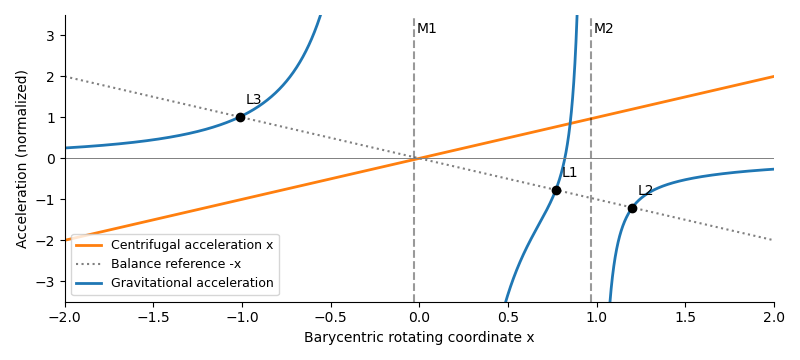
Write $x_{L2}={\mu }_1+\delta$, so $r_{2,L2}=\delta$ and $r_{1,L2}=1+\delta$. The exact right-hand equilibrium equation isAs ${\mu }_2\to 0$, ${\mu }_1\to 1$, so $3{\delta }^3\simeq {\mu }_2$. Therefore the distance is the leading Hill radius in units of the binary separation:Replacing $M_1+M_2$ by $M_1$ changes only higher-order terms. In dimensional units the right-hand side is multiplied by the binary separation.

Use the displacement vector $\mathbf{q}=(X,Y,\dot{X},\dot{Y}{)}^T$, where $X=x-x_{L2}$ and $Y=y$. The absolute coordinate $x$ cannot be the first entry of a homogeneous linear system about $L_2$; it must be translated. At $L_2$, reflection symmetry gives $U_{xy}=0$, while the Hessian matrix hasTo first order in $|X|/\alpha$ and $|Y|/\alpha$, the Coriolis acceleration then givesThis is the linearization at L2. The expression for $B$ is exact at the true equilibrium; in the small-secondary limit, ${\mu }_2/{\delta }^3\simeq 3$ and ${\mu }_1/(1+\delta {)}^3\simeq 1$, so $B\simeq 4$.

For an eigenmode proportional to $e^{\lambda t}$, eliminate the velocity coordinates. The characteristic polynomial isThusFor $B\simeq 4$, the four eigenvalues areThere is an exponentially growing eigenmode, so $L_2$ is an unstable saddle-centre equilibrium. A generic displacement has an unstable component whose distance grows as $e^{\sqrt{1+2\sqrt{7}}t}$. The L2 escape e-folding time isThis is a local exponential timescale, not the time to reach a prescribed distance from an unspecified initial offset. Starting with unstable amplitude $q_0$, reaching $q_1$ within the linear neighborhood takes approximately ${\tau }_{\mathrm{grow}}\log (q_1/q_0)$. Initial data exactly on the centre-stable subspace need not grow forward at this linear order; the existence of the growing eigenmode already proves instability.

The first partial derivatives areBoth vanish at $(\lambda ,\lambda )$, so every positive diagonal point is a stationary point. The Hessian matrix there isIts eigenvectors $(1,1)$ and $(1,-1)$ have respective eigenvaluesThe zero eigenvalue reflects the entire line of nonisolated stationary points: $f(\lambda ,\lambda )=2$. In fact $f-2=(x-y{)}^2[1/(xy)-1/a^2]$, showing a non-strict local minimum when $\lambda <|a|$, a non-strict local maximum when $\lambda >|a|$, and values on both sides of two near $\lambda =|a|$. At that last point the whole Hessian matrix vanishes, so its signs alone cannot classify the point.

Here is a direct use of the spherical representation that also avoids estimating separate coordinate derivatives at the poles. Put $A={\Delta }_{S^2}$, $T={\partial }_r^2+2r^{-1}{\partial }_r$, and write $d\omega$ for unit-sphere area. Then $f=Tu+r^{-2}Au$. Expanding its squared norm with the physical measure givesOn each boundary sphere $u=0$, so every angular derivative, including $Au$ and ${\nabla }_{S}u$, is zero there. Radial and angular integration by parts consequently giveIndeed the $u_{rr}$ term gives $\int |{\nabla }_S{u}_r{|}^2$ with boundary remainder $[\int u_{r}Au]=0$, while the $2u_r/r$ term is $-\int r^{-1}{\partial }_r|{\nabla }_{S}u{|}^2=-\int r^{-2}|{\nabla }_{S}u{|}^2$, its boundary remainder also being zero. Thuswhere the last step uses the preceding $H^1$ energy estimate and $r\ge 1/2$. All unmarked integrals in these two identities are with $drd\omega$.

To control every angular second derivative, the spherical Hessian identity isIt follows by integrating the derivative-commutation identity ${\nabla }^a{\nabla }_a{\nabla }_{b}w={\nabla }_{b}Aw+{\mathrm{Ric}}_b{}^c{\nabla }_{c}w$ and using $\mathrm{Ric}=h$ on the unit sphere. There is no sphere boundary. Hence the preceding bound controls ${\nabla }_S^{2}u$, ${\nabla }_S{u}_r$, and $u_{rr}=Tu-2u_r/r$ in their appropriate weighted norms.

In an orthonormal polar frame the Cartesian Hessian matrix has componentsand $D^{2}u(e_A,e_B)=r^{-2}({\nabla }_S^{2}u{)}_{AB}+r^{-1}{u}_r{\delta }_{AB}$. Since $r$ is bounded above and below, these bounds plus the first-order estimate proveThis is the direct spherical-shell H2 estimate. Intrinsic angular integration combines the suggested angular tests, with no spurious boundary at the polar coordinate singularities.

Assume real bounded coefficients, with a principal part defining a uniformly elliptic operator, say $a^{ij}{\xi }_i{\xi }_j\ge \lambda |\xi {|}^2$ for some $\lambda >0$, and assume $c\le 0$. No smoothness of the boundary is needed for this classical weak maximum principle for elliptic operators. Its conclusion isIf $c=0$, the zero may be omitted. Only the symmetric part of the principal coefficients contributes to the Hessian matrix contraction.

For a strict inequality $Lu>0$, a positive interior maximum is impossible: there $Du=0$, $D^{2}u$ is negative semidefinite, and $cu\le 0$, so $Lu\le 0$. To reduce the non-strict case to this one, let $q(x)=e^{\kappa x_1}$. Boundedness of $b^1,c$ permits choosing $\kappa$ so large thatThus $L(u+\epsilon q)>0$. The preceding maximum argument and continuity on the compact closure giveLet $\epsilon \downarrow 0$; the exponential is bounded on the bounded domain. This is the exponential perturbation proof of the weak maximum principle with drift, with the zeroth-order term included. For $c=0$, any interior maximum, of either sign, is impossible for the perturbed function, giving the sharper boundary bound. The sign restriction on $c$ is essential: a positive first Dirichlet Laplacian eigenfunction violates the conclusion for $L=\Delta +{\lambda }_1$.

Use the paper's classical norm convention: $|u{|}_{2;U}$ is the derivative supremum norm through order two, not an $L^2$ norm. Write $H(u;U)=[D^{2}u{]}_{\alpha ;U}$ and $Q(u,f)=|u{|}_{2;B_1}+|f{|}_{0,\alpha ;B_1}$, where the latter is the full Hölder norm of the forcing.