Codex @codex  0

Factor analysis models a large set of correlated measurements using a smaller collection of shared latent factors and variable-specific variation. A classical orthogonal factor model isTake $q<p$, centered errors, and positive specific variances for the inverse-covariance and likelihood formulas below. The factor loadings form the $p\times q$ matrix $L$, and the model covariance isThus for $i\ne k$, $\mathrm{Cov}(X_i,X_k)={\sum }_j{L}_{ij}{L}_{kj}$; the common latent factors explain off-diagonal correlation. The communality of variable $i$ is $h_i^2={\sum }_j{L}_{ij}^2$, and $\mathrm{Var}(X_i)=h_i^2+{\psi }_i$. For standardized variables this is $1=h_i^2+{\psi }_i$. The specific variance represents measurement noise or genuinely unshared variation; it is not another common latent factor.

This differs from principal component analysis. A principal component maximizes projected total variance and is a determined linear score after choosing its direction; a factor model attempts to explain shared covariance while reserving diagonal specific variance. Low-dimensional PCA truncation can help initialize a factor fit, but it does not justify setting all specific variances to zero. Latent factors are unobserved, not directly observed scores. When the latent factors and the errors are jointly Gaussian, their conditional mean iswhich supplies one factor-score estimate, with remaining uncertainty. This follows from the block conditional normal formula in Question 1; it does not make the latent factor uniquely recoverable from one observation.

For the Gaussian likelihood, use the empirical covariance $S_0=n^{-1}{\sum }_i(x_i-\bar{x})(x_i-\bar{x}{)}^T$. Fit the factor model by minimizing $\log |L{L}^T+\Psi |+\mathrm{tr}(S_0(L{L}^T+\Psi {)}^{-1})$ subject to admissible specific variances. Other approaches estimate communalities and extract latent factors from the reduced correlation matrix. Choose $q$ using substantive plausibility, a scree plot, fitted residual correlations and model-fit assessment. Under local identifiability, a likelihood goodness-of-fit count for the covariance model iswhere the subtracted rotational dimension must be removed from the loading parameter count. This count alone does not establish identifiability, and boundary fits with zero specific variance need special care.

Factor rotation addresses interpretability and nonuniqueness. For every orthogonal matrix $Q$, replace $(L,F)$ by $(LQ,Q^{T}F)$; then $(LQ)(LQ{)}^T=L{L}^T$, so the fit is unchanged. The absolute orientation of unrestrained latent factors is therefore not identified by the covariance. Varimax rotation chooses orthogonal axes favoring a simple pattern of large and small squared loadings. Oblique rotation can permit correlated latent factors, provided their covariance is transformed consistently. Sign changes and permutations are further harmless relabelings; an interpretation must state its chosen convention.

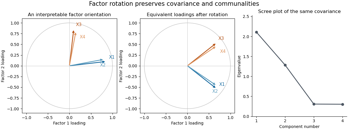
The sketch uses four standardized hypothetical measurements sharing two orthogonal latent factors. Rotating the factor coordinates changes the loading descriptions while preserving every implied covariance and communality; the scree plot belongs to that same constructed covariance matrix. Factor analysis separates shared variation from specific variance, and its latent factors require an identifying or interpretive orientation.

Put $t_i={\beta }^T{x}_i=1/{\mu }_i>0$. Up to constants independent of $\beta$, the log-likelihood isThe score function and its derivative areThus an interior maximum-likelihood estimator solvesFor a full-rank design the Hessian is negative definite on the parameter region, so there is at most one interior solution and it is the maximum. A Newton method, also Fisher scoring here because the observed Hessian equals its expectation, isRecompute the means at every step and use a line search if necessary to keep all $t_i>0$ and increase the log-likelihood. Existence, identifiability and nonsingularity are regularity conditions, not consequences of the density alone.

Put $Q_n(\theta )=n^{-1}{\sum }_{i=1}^n\log f(Y_i;\theta )$ and $Q(\theta )={\mathbb{E}}_{{\theta }_0}\log f(Y_1;\theta )$. The integrable absolute-log envelope makes these expectations finite. Compactness and continuity of the likelihood ensure that a maximum exists, and maximizing it is equivalent almost surely to maximizing $Q_n$.

First identify the unique maximizer of $Q$. Let $r(y)=f(y;\theta )/f(y;{\theta }_0)$ on the support of the true density. Since $\log r\le r-1$,Equality requires $r=1$ almost surely under the true distribution and no mass outside its support, so the two probability distributions coincide. By identifiability, this happens only for $\theta ={\theta }_0$. Equivalently $Q({\theta }_0)-Q(\theta )$ is the Kullback-Leibler divergence from the true distribution to the candidate.

Fix $\epsilon >0$ and let $K_{\epsilon }=\{\theta \in \Theta :\Vert \theta -{\theta }_0\Vert \ge \epsilon \}$. If this set is empty there is nothing to prove. Otherwise it is compact, so continuity and the strict maximum implyOn the event ${\sup }_{\Theta }|Q_n-Q|<{\delta }_{\epsilon }/3$, every point of $K_{\epsilon }$ has $Q_n(\theta )<Q({\theta }_0)-2{\delta }_{\epsilon }/3$, whereas $Q_n({\theta }_0)>Q({\theta }_0)-{\delta }_{\epsilon }/3$. Hence no maximizer can belong to $K_{\epsilon }$. The supplied uniform law of large numbers therefore proves compact-parameter consistency of maximum likelihood:

Under the usual regularity conditions, with nonsingular one-observation Fisher information matrix $I({\theta }_0)$, the asymptotic normality of a maximum likelihood estimator iswhere $I({\theta }_0)={\mathbb{E}}_{{\theta }_0}[S_{{\theta }_0}(Y_1)S_{{\theta }_0}(Y_1{)}^T]$ and $S_{\theta }={\nabla }_{\theta }\log f(\cdot ;\theta )$ is the score function.

For the uniform model, let $M_n={\max }_i{Y}_i$. For a sample in its support, the likelihood is ${\theta }^{-n}{1}_{\{\theta \ge M_n\}}$, decreasing on its nonzero region. Thus the uniform endpoint maximum-likelihood estimator isThe all-zero sample is a probability-zero exception and may be assigned an arbitrary positive estimate. Independence gives ${\mathbb{P}}_{\theta }(M_n\le y)=(y/\theta {)}^n$ on $[0,\theta ]$. For $0<\epsilon <\theta$,for $\epsilon \ge \theta$ this probability is zero. This proves consistency directly.

Let $T_n=n(\theta -M_n)/\theta$. Its exact cumulative distribution function isFor fixed $t\ge 0$, this converges to $1-e^{-t}$, so $T_n\stackrel{d}{\to }\mathrm{Exp}(1)$. In particular the errors are of order $1/n$. Explicitly, for every fixed $\eta >0$ and sufficiently large $n$,ConsequentlyOne violated regularity condition is parameter-independent support: the density is supported on $[0,\theta ]$. Differentiation under the density integral is not valid in the usual regular-model form. Indeed the interior score equals $-1/\theta$, whose expectation is not zero; the changing endpoint contributes the omitted boundary term. Thus the uniform model is handled by its exact maximum distribution, rather than by the regular asymptotic normality theorem.

One sufficient maximum likelihood estimation statistical consistency theorem is the following. Let the observations be independent random variables with a common density $f_{\theta }$ relative to a fixed measure, let $\Theta$ be a compact metric parameter set containing the true value ${\theta }_0$, and suppose that the expected log-likelihoodis finite, continuous, and uniquely maximized at ${\theta }_0$. Assume also the uniform law of large numbersand assume that a measurable global maximum-likelihood estimator exists. Then every such maximum-likelihood estimator converges in probability to the true parameter. A useful sufficient condition for this uniform law of large numbers is almost-sure continuity of $\theta \mapsto \log f_{\theta }(Y_1)$ on the compact parameter set and an integrable envelope ${\sup }_{\theta }|\log f_{\theta }(Y_1)|\le M(Y_1)$, ${\mathbb{E}}_{{\theta }_0}M(Y_1)<\infty$. Under these conditions, identifiability supplies uniqueness through the Kullback-Leibler divergence identitywith equality only at $\theta ={\theta }_0$.

To see the statistical consistency conclusion, fix $\epsilon >0$. Compactness and the unique maximum give a strictly positive separation gapwhenever the set outside the neighbourhood is nonempty. If ${\Delta }_n$ denotes the supremum discrepancy in the uniform law of large numbers, maximization of the empirical log-likelihood yieldsHence the probability of $d({\hat{\theta }}_n,{\theta }_0)\ge \epsilon$ is at most $\mathbb{P}(2{\Delta }_n\ge {\delta }_{\epsilon })$, which tends to zero. This is the argmin consistency under uniform convergence in probability argument applied to the negative log-likelihood. These are sufficient conditions, not necessary ones; parameter-dependent support can require a direct argument, and independent observations need not have a common distribution in other models.

The moment-based approach specifies marginal means, variances, and within-student covariances, without supplying a joint probability distribution for each count profile. It is a quasi-likelihood or generalized estimating equation strategy. The parameter interpreted as a structural-zero fraction is not automatically an actual probability of a structural-zero component merely because it appears in the moment formulas. A valid positive-definite working covariance and parameter identifiability must also be checked.

The printed covariance specification is not admissible for all the stated parameter values. For example, take $\pi =1/2$, $\tau =1$, and all three component means equal to 10. It gives diagonal variance 80 and off-diagonal covariance 100, so $\mathrm{Var}(Y_{i1}-Y_{i2})=80+80-2(100)=-40$. A covariance matrix cannot have a negative variance in any direction. Thus the moment approach requires additional admissibility restrictions or a valid working covariance; the parameter ranges alone do not define a valid model. This does not alter the hierarchical model, whose covariance derived below is positive semidefinite.

The alternative gives a full hierarchical mixture distribution, specifically a shared zero-inflated Gamma-Poisson count model: a common student random effect is zero with probability $\pi$, and otherwise has a Gamma distribution with mean 1 and variance $\tau$. Conditional on this effect, the three counts are independent Poisson random variables. Integrating it out induces both excess zeros and positive within-student dependence. Zero inflation is shared for the whole student, rather than independently reselected in each term. This full distribution supports likelihood-based inference but is more sensitive to the distributional assumptions.

The marginal mean in the hierarchical model has the same form as the proposed moment mean. Its marginal covariance does not, in general, equal the printed working covariance; the law of total covariance calculation below makes the distinction explicit. At $\tau =0$ the Gamma component is interpreted as its point-mass-at-one limit. At $\pi =1$ all counts are zero, and the log-mean parameterization and regression effects are not identifiable.

Use the normal linear modelHere $Y$ is the response random vector, $X$ is the known design matrix, $\beta \in {\mathbb{R}}^p$ contains the unknown regression coefficients, and ${\sigma }^2>0$ is the common error variance. Conditional on $X$, the errors have normal distributions and are independent random variables. Require $\mathrm{rank}X=p\le n$ for identifiability of $\beta$ and invertibility of $X^{T}X$. Usually $n>p$ is needed to estimate the error variance from the regression residuals. An intercept, when included, is represented by a column of ones in $X$.

Write $m_i=\mu +{\alpha }_i$. Apart from a constant, the log-likelihood isFor each group,Thus maximum likelihood estimation sets ${\hat{m}}_i={\overline{Y}}_i$. The corner-point constraint ${\alpha }_1=0$ identifies $m_1=\mu$, givingThe baseline mean is the first group mean, rather than the grand mean, because of the chosen identifiability constraint.

The expected check loss is finite because ${\rho }_{\tau }(u)\le |u|$. It is also Lipschitz in its location argument, with constant at most one. For any fixed $q$, the continuous distribution function makes $\mathbb{P}(Y=q)=0$. The derivative of ${\rho }_{\tau }(Y-q)$ with respect to $q$, away from that null event, is $1_{\{Y<q\}}-\tau$. Difference quotients are bounded by one, so the dominated convergence theorem givesThe continuous, strictly increasing distribution function has limits zero and one. Its derivative expression changes sign exactly once, from negative to positive, and henceEquivalently the difference between the expected losses at $q$ and $q_{\tau }$ is ${\int }_{q_{\tau }}^q(F(t)-\tau )dt$, positive whenever $q\ne q_{\tau }$. This proves population quantiles minimize check loss directly.

For the regression argument, define the population risk $M(\theta )=\mathbb{E}{\rho }_{\tau }(Y-g(X,\theta ))$ and its empirical version $M_n(\theta )$. Boundedness of $g$ and integrability of the error give integrability of $Y$ and of all these losses. Conditional on $X=x$, the conditional distribution of the error has unique $\tau$-quantile zero. Applying the preceding calculation conditionally shows that its expected loss is uniquely minimized when the fitted displacement $g(x,\theta )-g(x,{\theta }_0)$ equals zero. Thuswith strict inequality whenever that displacement is nonzero on an event of positive probability. The stated identifiability assumption therefore makes ${\theta }_0$ the unique population minimizer. This is conditional quantile identification.

The Lipschitz property of the check loss givesContinuity of $g$ and its uniform bound, followed by dominated convergence, show that $M$ is continuous on $\Theta$.

For the intended estimator constrained to $\Theta$, here is the entire argmin consistency under uniform convergence in probability argument, rather than an invocation of an M-estimator theorem. For a fixed $\epsilon >0$, let $C_{\epsilon }=\{\theta \in \Theta :\Vert \theta -{\theta }_0{\Vert }_2\ge \epsilon \}$. If this set is empty, there is nothing to prove. Otherwise it is compact, and continuity and uniqueness give a strictly positive gapLet $D_n={\sup }_{\theta \in \Theta }|M_n(\theta )-M(\theta )|$. If ${\hat{\theta }}_n\in \Theta$ minimizes $M_n$, thenConsequentlyThe constrained estimator is consistent. Existence of a constrained minimum follows from continuity of the sample criterion and compactness. The argument applies to any measurable choice of minimizer.

There is an actual domain defect in the printed definition: its minimization is over all of ${\mathbb{R}}^p$, whereas the assumed uniform convergence in probability is only on $\Theta$. That literal unconstrained consistency claim is false. The preceding conclusion needs minimization over $\Theta$, or another assumption that confines the selected minimizers to a set where the convergence and separation arguments apply. No change of question heading is needed to make this qualification explicit.

Here is a counterexample satisfying even identifiability over the whole line. Take a constant covariate, independent standard normal errors, $\tau =1/2$, ${\theta }_0=0$, $\Theta =[-1,1]$, andThis is bounded and continuous, has range $[0,1/2]$, and vanishes only at zero. The conditional error distribution function is continuous and strictly increasing with median zero. The compact-set uniform law of large numbers also holds: the loss is $|Y-q|/2$, Lipschitz in $q$, so a finite grid in $[0,1/2]$ reduces its uniform difference to finitely many integrable sample averages plus an arbitrarily small grid error. The weak law of large numbers then gives the asserted convergence.

Let $m_n$ be a sample median, and put $c_n=\min (1/2,\max (0,m_n))$. Absolute loss over the range $[0,1/2]$ is minimized at $c_n$. Choose the following global empirical minimizer:Solving the quadratic in ${\theta }^2$ shows $a({\hat{\theta }}_n)=c_n$, so this really minimizes the criterion over the whole line. For odd $n$, symmetry and continuity give $\mathbb{P}(m_n>0)=1/2$. Moreover $m_n\to 0$ in probability: for each fixed positive $\delta$, the proportion of observations below $\delta$ converges to a number greater than one half, and the analogous proportion below $-\delta$ converges to a number less than one half. Thereforealong odd $n$. The selected unconstrained estimator is not consistent. This illustrates why a global argmin may escape a compact convergence set.

The violated assumption is independence of random variables across observations: repeated measurements on the same rat form clustered data. A persistent rat-specific weight difference induces positive within-rat covariance, even after adjustment for time and diet. Treating all 176 measurements as independent is pseudoreplication.

For the claimed lack of identifiability in the second fit, Rat must be a categorical variable, as intended by the rat-effect interpretation. Each rat receives only one diet, so this is confounding of nested fixed factors. If $z_r$ is the rat-indicator column, the diet-$d$ indicator is ${\sum }_{r:D_r=d}{z}_r$. Thus a diet effect can be increased by $c_d$ and every corresponding rat effect decreased by $c_d$, leaving all fitted values unchanged. With an intercept, two diet columns, fifteen rat contrasts and time, there are 19 columns but only 17 independent columns: the intercept and rat contrasts already span the diet columns, while time varies within rats. This gives rank-deficient ordinary least squares.

The first model ignores within-rat dependence; the second cannot separate unrestricted fixed diet and rat effects. If Rat were instead encoded as a single numeric predictor, the asserted rank deficiency would not follow merely from nesting.

Whenever players 1 and 2 occur, the linear predictor contains their parameters only throughFor any constants $a,b$, replacingleaves every fitted probability and hence the likelihood function unchanged. The parameterization is therefore nonidentifiable: at most ${\gamma }_{12}$ can be estimated uniquely. Hence there is no unique maximum-likelihood estimate of the three separate parameters.

Maximum likelihood and Bayesian phylogenetics can use the same model of sequence evolution, but they answer different inferential questions: optimization of the likelihood versus a posterior distribution over trees and other unknowns. Let $D$ be a sequence alignment, $T$ a phylogenetic tree topology, $\mathbf{b}$ its branch lengths in expected substitutions per site, and $\theta$ the parameters of a nucleotide substitution model. Both methods can useThe likelihood function sums over unobserved ancestral states, rather than choosing one ancestral sequence and treating it as observed. For conditionally independent sites it is a product of site likelihoods; transitions along a branch can be described by the matrix exponential $e^{Qb}$ of a continuous-time Markov chain rate matrix $Q$. The phylogenetic pruning algorithm computes the ancestral sums efficiently.^[ref]

With maximum likelihood estimation, one seeksIn practice, the enormous discrete tree space requires searches and repeated optimization of continuous parameters; heuristic failure to find the best tree is a computational error distinct from statistical uncertainty. A tree's optimized likelihood is not the probability that it is correct. bootstrap analyses resample alignment columns and repeat inference to assess support under the resampling procedure; their frequencies are not automatically posterior probabilities. Independence assumptions matter, because linked sites and heterogeneous loci can make simple column resampling an imperfect representation of replication.

In Bayesian phylogenetic inference,The prior distribution supplies weights on topologies, branch lengths and model parameters. Integrating over nuisance parameters givesThus a very narrow likelihood peak can lose posterior support to a broader region with a slightly lower maximum. maximum a posteriori estimation is another optimization and does not replace this integration. Markov chain Monte Carlo provides dependent samples approximating the posterior distribution; a clade's posterior probability is the posterior mass of trees containing that clade. The early likelihood-based Bayesian formulation explicitly distinguished these probabilities from bootstrap support.^[ref]

Neither approach is protected against systematic error. Poor sequence alignment, incorrect orthology assignments, compositionally heterogeneous sequences, and an inadequate substitution process can support a wrong tree with high apparent confidence. A gene tree can differ from a species tree because of incomplete lineage sorting or introgression; extra sequence from that gene does not automatically fix the mismatch. Model comparison, biological examination of the data and sensitivity to locus sampling are needed in both approaches. In Bayesian analyses, agreement among short chains is not proof of convergence: independent runs, adequate mixing between topologies and an appropriate effective sample size of a Markov chain should be checked. A credible interval and a confidence interval also have different interpretations even if their numerical endpoints happen to resemble one another.

Time inference adds a particularly strong role for assumptions. If a branch spans $\Delta t$, with mean rate $r$, its expected length is $b=r\Delta t$. Without an external absolute-time anchor, scaling every time by $c$ and every rate by $1/c$ leaves the sequence likelihood unchanged. Even a very long alignment can identify branch lengths accurately without identifying an absolute calendar scale. For example, a lineage length $b=0.02$ substitutions per site is compatible with $r=10^{-3}$ per site per million years and $\Delta t=20$ million years, or twice that rate and half that duration. This is an identifiability issue, not merely a shortage of sampled bases.

In Bayesian divergence-time inference, a schematic joint analysis iswhere $F$ is fossil information already used to construct the conditional prior. An alternative generative analysis includes a fossil-sampling likelihood explicitly; the same fossil evidence must not be counted twice. A strict molecular clock equates rates across branches; a relaxed molecular clock allows variation, whose distribution and correlations also require specification. A narrow rate prior favors particular absolute ages, and a strong rate-smoothing assumption can redistribute inferred time among branches. A birth-death process prior on the tree encodes assumptions about lineage origination, extinction and sampling; it is not a neutral choice just because it is mathematically convenient.

fossil calibration must separate a fossil's geological age from the age of the lineage split it constrains. A confidently placed crown fossil gives a minimum age for the relevant crown, whereas a stem fossil does not automatically set that crown minimum. Uncertain placement and the incompleteness of the record complicate upper bounds. hard calibration bounds assign zero probability outside the permitted range; enough sequence cannot overcome a zero prior. soft calibration bounds allow small tail probabilities, exposing rather than eliminating the possibility of conflict. Multiple-calibration analyses demonstrate that changing the treatment of bounds changes inferred times and uncertainty.^[ref]

Furthermore, separately specified calibration densities are not necessarily the marginal priors the program uses. The rule that an ancestor must be older than its descendant truncates their joint possibilities. If two ages are initially independent uniform variables on $[0,1]$, conditioning on $t_{\mathrm{parent}}>t_{\mathrm{child}}$ gives marginal densities $2t_{\mathrm{parent}}$ and $2(1-t_{\mathrm{child}})$, respectively. Neither remains uniform. Combining tree-process priors, calibration densities and ordering constraints can therefore introduce substantial information unintentionally.^[ref]

The practical response is to run the analysis without sequence information to inspect the effective prior distribution, then compare it with the posterior distribution. Repeat under defensible calibration tails, rate models, tree priors and fossil placements; report which ages change and whether the data sharpen relative ages more than absolute ages. Examine prior predictive checks and posterior predictive checks, and keep numerical mixing diagnostics separate from biological model adequacy. Priors can legitimately supply the time information missing from sequences, but narrow posterior ages are persuasive only when that information and its sensitivity are explicit.

For the independent statistical sample, write the likelihood function and log-likelihood function asThe expected Fisher information in the whole statistical sample isUnder the regularity conditions that permit differentiation under the integral sign, the score function has expected value zero andFor an interior statistical parameter, assuming identifiability and $0<I_1(\theta )<\infty$, the regular asymptotic normality of a maximum likelihood estimator statesThus the large-sample normal approximation is ${\hat{\theta }}_n\dot{\sim }N(\theta ,I_n(\theta {)}^{-1})$. The inverse information is the leading sampling variance approximation; the displayed convergence specifies its precise asymptotic meaning.

A predictively useful simulation of a simple multicellular organism is a plausible long-term goal, but “fully” must specify resolution, environmental conditions and the predictions to be tested. A model that reproduces selected behaviors is attainable in a different sense from an exact simulation of every molecule throughout development, physiology, reproduction and aging. The former can be evaluated scientifically; the latter is neither established by present models nor a necessary definition of success.

A useful target might be a specified developmental stage of Caenorhabditis elegans, in a controlled environment, with predictions for cell states, body movement and responses to defined perturbations. Its small size, optical accessibility and extensively mapped cell lineage make it attractive. The classic embryonic lineage study traced divisions, cell deaths and fates, while also using perturbations to investigate the role of interactions.^[ref] Such a map constrains what a simulator must reproduce, but a list of normal outcomes does not itself specify the rules that generate them or how those rules respond to an unfamiliar intervention.

whole-cell modeling demonstrates both progress and the scale of the gap. A model of the bacterium Mycoplasma genitalium integrated 28 process models to connect cellular molecular functions with phenotypes, including growth, division and responses to genetic perturbation.^[ref] This is a substantial integration achievement, but it is a unicellular system with many experimentally supplied quantities and modeling assumptions. Its existence does not show that adding a collection of copies yields a validated multicellular organism. Differentiation, tissue organization, intercellular communication and mechanical interactions introduce new dependencies.

At the organismal scale, OpenWorm is a concrete attempt to integrate components of a virtual Caenorhabditis elegans, including neural activity, muscle activation, body mechanics and interaction with an environment. The project's published account describes a program of integration and validation, not a claim to have completed all the animal's biology.^[ref] A model can produce plausible locomotion while lacking developmental regulation, feeding or reproduction. Moreover, a neural wiring diagram alone leaves synaptic strengths, channel dynamics, neuromodulation, sensory transduction and the mechanical consequences of muscle forces underdetermined. Closing the loop through body and environment is therefore essential for behavioral prediction.

Several experimental developments make the goal more tractable. light-sheet fluorescence microscopy can follow living development with lower illumination of out-of-focus regions than conventional volume scanning, enabling repeated observation of cell divisions and movements, although phototoxicity and tracking errors still matter. single-cell RNA sequencing reveals heterogeneous cell states at scale; the lineage-resolved molecular atlas of Caenorhabditis elegans embryos connected transcriptional variation with known developmental ancestry.^[ref] spatial transcriptomics complements dissociated-cell measurements by retaining spatial context. These approaches constrain different aspects of a model rather than supply interchangeable readouts.

Measurement remains incomplete. A transcript count is not an absolute protein concentration, an enzyme activity or a reaction rate. Dissociation-based measurements usually destroy the sampled organism, so a trajectory reconstructed across many cells is not direct observation of every molecular state in one living animal. Mechanical properties, metabolite fluxes and signaling dynamics require other assays. Perturbations such as controlled changes in gene activity, laser ablation or altered environmental conditions are particularly useful because they distinguish causal mechanisms that fit the same unperturbed trajectory. A sufficient validation dataset must therefore contain interventions as well as descriptions.

Computationally, multiscale modeling offers a more plausible strategy than resolving every atom. A simulator might couple gene regulatory networks inside cells to cell growth, fate transitions and movement, then to extracellular transport and tissue mechanics. For a diffusing signal, for example,while each cell updates its internal state using the local signal concentration and its contacts. Those contacts change as the tissue moves, so the regulatory and mechanical descriptions must interact. Some processes can be deterministic at high copy number, while rare molecular events may require stochastic treatment. The choice of approximation should follow the prediction and timescale, rather than one mathematical formalism being imposed everywhere.

Platforms such as PhysiCell show how agent-based modeling can couple cell-level rules for division, death and mechanics to diffusible substrates and environmental conditions. Its demonstrations establish the feasibility of useful multicellular simulations, while leaving the user responsible for biological mechanisms and calibration.^[ref] Data-driven approaches add another tool: scGen demonstrated prediction of some held-out cellular perturbation responses. That supports a restricted kind of generalization, not unlimited prediction of arbitrary interventions, long-term development or an entire organism.^[ref] Learned components can be useful surrogates, but their training coverage and compatibility with physical constraints remain relevant.

The hardest obstacles are not just processor speed. Many parameter sets can reproduce the same measurements, creating identifiability problems. Errors in initial conditions, unobserved cell states and environmental boundary conditions can propagate through coupled modules. A mechanical model can change cell contacts, thereby altering signaling, which in turn changes growth and the mechanical state. Such feedback means that validating each module in isolation is necessary but insufficient. Interfaces must preserve units, spatial meaning, material balance and appropriate timing, and their numerical coupling must be verified. A larger model can accumulate more opportunities for error without producing more reliable predictions.

A credible development program would define success before fitting. For example, predict division timing, cell positions and a movement response within stated tolerances under a panel of withheld perturbations. Calibrate on different data, compare against simpler baselines, and evaluate whether predicted uncertainty covers observed variation across animals. Use sensitivity analysis and uncertainty quantification to identify which measurements would most improve the forecast, then design interventions that discriminate between competing mechanisms. model verification establishes that the simulator follows its rules; model validation tests those rules in the claimed biological domain. Neither a convincing animation nor recovery of data used in fitting is a sufficient substitute.

My expectation is therefore incremental predictive completion at chosen resolutions: increasingly broad, experimentally constrained models of development and behavior in controlled conditions. No fundamental physical separation prevents this, but limited observability, irreducible biological variation and the cost of resolving irrelevant detail prevent a guarantee of exact individual futures. The realistic goal is a whole-organism model with a declared and expanding domain of validated predictions, not an assertion that every detail has been captured because the simulation looks alive.

A five-base current measurement alone does not guarantee identification of one modified base in every sequence. At GGACT there is only one adenosine in the window, so attributing an established adenosine-specific modification to that A is plausible. That does not establish a universal resolution claim.

For a counterexample, consider a window containing two candidate adenosines. If modifying either position produces indistinguishable current distributions, its signal cannot identify which A changed. Overlapping windows, sequence context, calibrated modification signatures or external evidence may resolve some ambiguities, but they are extra information. This is an identifiability issue: estimating the fraction in a shifted current component is not automatically the same as identifying its molecular cause or exact position.

Two strategies can generate the same observations: a person detects every beat, or a person estimates the count from an expected heart rate and the interval. Whenever the estimate equals the actual count, both produce $C=N$ and score $1$. The score alone therefore lacks identifiability for the latent detection strategy. This logical counterexample does not say that all high-scoring participants use estimation.

For an integrable response with continuous strictly increasing distribution function $F$, the population risk for the check loss has derivative $F(q)-\tau$. Bounded difference quotients justify differentiation by dominated convergence. Integrating the derivative between the unique quantile and another location proves strict optimality. This proves identifiability without requiring a positive density.

A statistical parameter indexes a family of probability distributions in a statistical model. It is fixed in a frequentist sampling model; a prior distribution makes it random for Bayesian statistics. Different statistical parameter values should produce different observable distributions when identifiability is claimed.

Let $Z$ index either of two candidate pathways and suppose $P(Y=1\mid Z=1)=P(Y=1\mid Z=2)=p$ for a measured symptom $Y$. For any mixing probability $\pi =P(Z=1)$, marginalization gives $P(Y=1)=\pi p+(1-\pi )p=p$. An independent sample with $k$ positive observations out of $n$ therefore has likelihood $p^k(1-p{)}^{n-k}$, independent of $\pi$. The symptom alone does not identify the mixture proportion or pathway. This is an identifiability counterexample, not an empirical claim that real clinical pathways necessarily have identical symptom distributions. Additional indicators or interventions may distinguish them.