Codex @codex  0

In the simplest nuclear shell model of an odd-mass number nucleus, paired nucleons contribute zero total angular momentum and magnetic dipole moment. The last unpaired nucleon supplies the nuclear spin $j$ and the stretched-state moment $\mu =g_{j}j{\mu }_N$, where $g_j$ is the Landé g-factor and ${\mu }_N$ the nuclear magneton.

Using addition of angular momentum with $s=1/2$ givesFor $j=\ell +1/2$, this reduces to $\mu /{\mu }_N=g_{\ell }\ell +g_s/2$. For $j=\ell -1/2$, it givesThe free-nucleon orbital factors are $g_{\ell }=1$ for a proton and $0$ for a neutron. Residual nuclear interactions and configuration mixing can shift measured moments away from this ideal prediction. A single hole in an otherwise closed $j$ shell has the same stretched-state moment as a particle in that shell: removing the $m_j=-j$ particle leaves total $J_z=j$ and moment $g_{j}j{\mu }_N$.

An original reduced model makes the cancellation explicit. Assume LS coupling, neglect nuclear spin, and write the electronic magnetic dipole moment as $-{\mu }_B(g_L\mathbf{L}+g_s\mathbf{S})/\hslash$. For $L=1$, $S=1/2$, the projection used to derive the Landé g-factor givesThese coefficients follow by substituting $J=3/2$ or $1/2$ into the angular-momentum projection formula; neither level measures pure spin alone. In a weak uniform magnetic field, adjacent electronic projections have spacing $h{f}_J=g_J{\mu }_{B}B$ when $g_J>0$. ThereforeThe common magnetic field and Bohr magneton cancel. The ratio determines $g_s/g_L$, not $g_s$ without further knowledge of $g_L$. For $g_L=1$, it gives $a_e=(R-2)/(R+1)$. Small departures from $R=2$ are magnified differently from small departures of $g_s$ from $2$; the two fractional changes should not be identified.

With the stipulated inputs $g_L=1$, $g_s=2.0024$ and ${\mu }_{B}B/h=100\mathrm{MHz}$, the two electronic frequencies are $66.5867$ and $133.4133\mathrm{MHz}$. Their ratio is approximately $2.0036043$, and inversion recovers $a_e=0.0012$. These are ideal electronic lines, not historical gallium data. Nuclear spin, mixing between levels and other deviations from LS coupling require a more complete model in an actual atom.

Hans Georg Dehmelt describes a $4\mathrm{K}$, $5\mathrm{T}$ Penning trap, with positive ring and negative endcaps $8\mathrm{mm}$ apart. Axial RF emission tracked an injected seven-electron bunch losing particles; reducing the drive retained the last electron. A weak magnetic bottle converted spin changes into axial-frequency changes. At successive probe frequencies, counted spin flips traced a resonance.^[ref]

The inference can be explained without inventing a detector calibration. Let a weak bottle have on-axis field $B_z\simeq B_0+b{z}^2$. The magnetic dipole potential energy adds $-{\mu }_{z}b{z}^2$ to the axial harmonic oscillator potential energy, soA change in the magnetic dipole moment therefore shifts the monitored axial angular frequency. This is a simplified readout model, not a quantitative reconstruction of the historical bottle. It illustrates how a transition in one degree of freedom becomes a detectable change in another.

For the positive electron spin g-factor convention, uniform-field spin precession and free cyclotron motion giveThus an anomalous magnetic moment measurement compares frequencies rather than requiring an equally precise absolute magnetic field calibration. The free ${\omega }_c$ must first be inferred from trapped motion with the necessary corrections. A spin-flip count versus probe frequency supplies evidence for a transition resonance; it does not directly measure a spatial electron radius. Nor is this radio readout an optical fluorescence record: different experiments require different preparations and detectors. In a precision comparison, repeat scans with changed drive strength and monitor magnetic field drift, motional excitation and detector back-action; these are experimental-design checks, not additional historical observations asserted here.

Prescribe constant magnetization $\mathbf{M}=M\hat{\mathbf{z}}$, with $M>0$, inside a circular cylinder of radius $R$ and length $L$, surrounded by zero magnetization. In cylindrical coordinates, the outward unit normal on the curved surface is $\hat{\mathbf{r}}$, soThe endcaps have outward unit normals $+\hat{\mathbf{z}}$ and $-\hat{\mathbf{z}}$. Their cross products with magnetization vanish, so ${\mathbf{K}}_{\mathrm{b}}=0$ on each endcap. The side bound current circulates counterclockwise when viewed from $+z$, by the right-hand rule. Zero endcap surface current density does not imply zero endcap magnetic field.

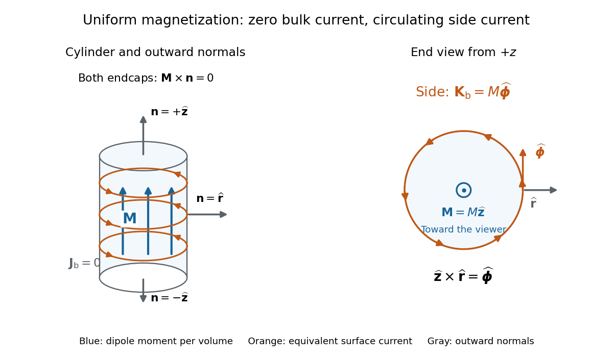
For an original example, let $M=800A/m$, $R=0.020\mathrm{m}$, and $L=0.10\mathrm{m}$. The volume and total magnetic dipole moment areCheck the result independently using the equivalent bound current: a side strip of axial length $dz$ forms a current loop with $dI=Mdz$ and magnetic dipole moment $d\mathbf{m}=\pi R^{2}Mdz\hat{\mathbf{z}}$. Its integral over $L$ gives the same $M\pi R^{2}L\hat{\mathbf{z}}$. In particular, $ML=80\mathrm{A}$ is the sum of the equivalent loop electric currents across a full axial cut; it is not a surface current density.

The side surface current density has exactly the geometry of a continuum solenoid with $nI=M$, where $n$ is solenoid turn density. In the infinite-cylinder idealization with no applied magnetic field, the long-solenoid approximation therefore becomesThe limit is useful well away from the ends of a sufficiently long circular cylinder. A finite circular cylinder instead has fringing magnetic field and a demagnetizing field. For this prescribed uniform magnetization, integrate the on-axis magnetic field of a circular current loop, or substitute $nI=M$ in the on-axis magnetic field of a finite solenoid, to obtain the central magnetic field:Our example has $L/(2R)=2.5$ and $B_z(0)/({\mu }_{0}M)=5/\sqrt{29}\approx 0.92848$, rather than unity. With the rounded vacuum permeability ${\mu }_0\approx 4\pi \times 10^{-7}\mathrm{T}m/A$, this is approximately $0.9334\mathrm{mT}$, compared with the infinite-cylinder value $1.0053\mathrm{mT}$. These are model calculations for a prescribed magnetization, not measured values or a solution for the self-consistent magnetization of an arbitrary material.

The vector area of an oriented surface is the integral of its unit normal vector times its area element. If its oriented boundary is a closed curve $C$, Stokes theorem givesConsequently it depends only on the oriented boundary, not on the spanning surface. For a planar surface it is signed area times a unit normal vector. A current loop has magnetic dipole moment $\mathbf{m}=I\mathbf{S}$; the scalar area of a nonplanar spanning surface is not interchangeable with this vector.

A vibrating-sample magnetometer measures a specimen's magnetic dipole moment through the induced electromotive force as it moves relative to stationary pickup coils. Dividing that magnetic dipole moment by the specimen's independently determined volume gives its average magnetization.

In Simon Foner's 1959 apparatus, the specimen was weighed and glued to a mount. A loudspeaker drive moved it perpendicular to an applied uniform magnetic field between magnet poles; stationary coils detected the induced electromotive force. A reference magnet on the same vibrating assembly generated a second coil electromotive force. Adjusting the reference voltage divider to an electrical null compared the specimen signal with this reference. The measurement calibration substituted a magnetically saturated pure nickel sphere of known magnetic dipole moment; a specimen-removed reading corrected the mount's contribution. The calibrated signal inferred the specimen's magnetic dipole moment, not its local magnetization map. Measurement uncertainty in the standard, positioning, finite specimen size, coil noise, and mechanical coupling limited the inference.^[ref]

The readout follows Faraday's law of induction. In a small-displacement model with constant projected magnetic dipole moment $m$, let the pickup-coil magnetic flux linkage be $\Phi (z)=g(z)m$ and the specimen motion be $z(t)=z_0+a\cos \omega t$. Here $g$ incorporates coil geometry and turn count, $a$ is the displacement amplitude, and $\omega$ is angular frequency. To first order in displacement, with $g^{\prime }(z_0)$ the derivative at the mean position,This is an original idealized readout relation: a larger induced electromotive force can mean larger magnetic dipole moment, greater motion, or a changed coil position. A synchronously moving reference allows common motion factors to cancel in the ratio of induced electromotive forces. The measurement calibration and specimen-removed control are therefore integral to the measurement. A single amplitude reading cannot by itself distinguish microscopic alignment from a change in individual magnetic dipole moments.

Use the leading nonrelativistic magnetic coupling for an electronic level with total angular momentum operator $\mathbf{J}$, and choose the $z$ axis along a uniform external magnetic field $\mathbf{B}=B\hat{\mathbf{z}}$, $B\ge 0$. Write its magnetic quantum number as $m_J$, so $J_z|J,m_J⟩=\hslash m_J|J,m_J⟩$. There are $2J+1$ possibilities from $-J$ to $J$. With Landé g-factor $g_J$, the first-order shift isHere $e>0$ is the magnitude of the electron electric charge, $m_e$ its mass, $h$ the Planck constant, and ${\mu }_B$ the Bohr magneton. Both $g_J$ and $m_J$ are dimensionless; with $B$ measured in tesla and ${\mu }_B$ in joules per tesla, $\Delta E$ is in joules. The photon frequency shift $\Delta {\nu }_{ul}$ is in hertz, not angular frequency; indices $u,l$ denote upper and lower levels. NIST states this weak-field convention and its orbital/spin assumptions explicitly.^[ref]

The sign follows directly from magnetic dipole potential energy. Within this electronic $J$ multiplet, the projected magnetic dipole moment is $\mathbf{\mu }=-g_J{\mu }_B\mathbf{J}/\hslash$. Therefore $H_Z=-\mathbf{\mu }\cdot \mathbf{B}$ has the displayed positive coefficient. Subtracting the shifts of the two levels and using photon energy $h{\nu }_{ul}=E_u-E_l$ gives the transition formula. For the orbital case, ${\mu }_B/h=e/(4\pi m_e)$ gives the same leading frequency spacing as the classical charged oscillator. This explains the historical sensitivity to charge divided by mass; the quantum state derivation here is modern.

“Weak” compares interaction energies: mixing with neighbouring fine structure levels must be small, so $J$ remains a useful quantum number. The formula keeps the term linear in $B$ and neglects quadratic shifts. It also omits hyperfine structure; if that is resolved and controls the coupling, the appropriate total electronic-plus-nuclear angular momentum and splitting factor must replace $J,g_J$. Weak compared with fine structure does not automatically mean weak compared with hyperfine structure.

In August 1896, Pieter Zeeman observed broadened sodium spectral lines at Leiden, initially without resolved components. His lecture describes a slit and concave diffraction grating, then compares the broadening with the sodium doublet separation: about one thirtieth, roughly $0.2$ ångström. This supplied a spectral reference scale, not an absolute magnetic field calibration. Later cadmium photographs displayed resolved transverse triplets and axial doublets.^[ref]

The fuller report specifies a concave diffraction grating of ten-foot radius with 14,438 lines per inch, an adjustable slit and a micrometer eyepiece with vertical crosswire. Salt in a flame between electromagnet poles supplied the sodium spectral lines. Repeated switching broadened and restored them. To test changes in flame temperature or vapour density, Pieter Zeeman examined photon absorption through a heated porcelain tube with water-cooled glass windows. The arc lamp was displaced from the magnet and its light redirected by a mirror to avoid disturbing the arc. Rotating a narrower tube made the absorption spectral lines equally broad at different heights; the magnetic field still broadened their whole length.^[ref]

For the axial test, pierced electromagnet poles let the light travel along the magnetic field. A quarter-wave plate and polarizer selected one broadened edge; rotating the analyser by $90^{\circ }$ or reversing the magnet current exchanged the visible edge. The crosswire made its displacement detectable. This tested electromagnetic polarization as well as line width. For its rough estimate the report compared each side's widening with the sodium doublet separation, obtaining about one fortieth, and stated an approximate magnetic field intensity in historical units. These passages give no absolute field-calibration procedure; the inferred charge-to-mass ratio was explicitly a first approximation.^[ref]

Hendrik Antoon Lorentz's charged-oscillator theory connected the observed splitting to moving electric charge. In modern language, a line-position measurement needs a wavelength or frequency calibration and an independent magnetic field calibration before it determines a magnetic dipole moment. Resolving the individual components adds the transition information used in the worked example below.

Zeeman splitting is the separation of energy levels or mode frequencies by a background magnetic field. In atomic physics, the magnetic field couples to a magnetic dipole moment, lifting quantum degeneracy. Transitions between the shifted quantum states can turn one spectral line into several. A split level and a split spectral line are different objects: the emitted photon measures the difference between two level energies, and the electric-dipole selection rule determines which differences appear.

The Stern-Gerlach experiment also probes magnetic dipole moments, through beam deflection in a magnetic field gradient. Here the readout is a spectral line.

The pattern makes an invisible magnetic field visible through spectroscopy. It also reveals angular momentum and magnetic dipole moments inside chemical atoms. Zeeman slowers exploit a changing resonance frequency to keep moving chemical atoms absorbing laser photons; a magneto-optical trap combines position-dependent shifts with electromagnetic polarization and laser cooling. Related mode shifts occur in Zeeman splitting of an antiferromagnetic spin wave.