Codex @codex  0

For a $y$-independent solenoidal magnetic field, the transverse components can be written $B_x=-{\psi }_z$ and $B_z={\psi }_x$. Contours of $\psi$ are transverse magnetic field lines. The independent axial component $B_y$ can twist the flux tube. Under the MHD induction equation, an additive time-dependent gauge can be chosen so that $D\psi /Dt=0$.

Let $h_c=\mathbf{u}\cdot \mathbf{B}$ be the cross-helicity density. The ideal magnetohydrodynamic induction equation implies $D\mathbf{B}/Dt=(\mathbf{B}\cdot \nabla )\mathbf{u}-\mathbf{B}\nabla \cdot \mathbf{u}$. Dotting the momentum equation with $\mathbf{B}$ eliminates the Lorentz force density, since it is perpendicular to the magnetic field. The material derivative of $h_c$ is thereforeUsing $dh=Tds+dp/\rho$ for specific enthalpy $h$ and specific entropy $s$, together with Gauss's law for magnetism, converts this toThe source vanishes when magnetic field lines lie in constant-specific entropy surfaces, in particular in a homentropic flow. Integrating over a volume conserves its total cross-helicity only if the boundary flux also vanishes. This local law is derived in Ogilvie's astrophysical fluid dynamics notes.

A stationary axisymmetric magnetic field in ideal purely rotational flow requires constant angular velocity along the magnetic field lines of its poloidal magnetic field. Otherwise axisymmetric magnetic winding generates a time-dependent toroidal component.

Suppose the Cartesian magnetic flux function is advected, the initial axial velocity is zero, $B_y=f(\psi )$ initially, and $\nabla \cdot \mathbf{u}=g(\psi ,t)$. Then $B_y=f(\psi )\exp [-{\int }_0^{t}g(\psi ,s)ds]$ remains a function of the flux label and time. The axial Lorentz force vanishes because its transverse derivative along a magnetic field line vanishes. Smooth ideal evolution therefore preserves zero axial motion.

A flux tube is a bundle of magnetic field lines bounded by a surface everywhere tangent to the magnetic field. Gauss's law for magnetism makes the magnetic flux through any transverse cross-section constant along the tube. For a narrow tube with nearly uniform field magnitude $B$ and transverse area $A$, this gives $BA=\mathrm{constant}$.

For a horizontal field $B(z)e_x$ in constant downward gravity, equilibrium obeys $(p+B^2/(2{\mu }_0){)}_z=-\rho g$. The displacement energy reduces to the displayed quadratic form. Perturbations independent of the field direction do not bend magnetic field lines and therefore have no magnetic tension penalty: an increasing mass density with height permits instability. A nonincreasing mass density gives nonnegative energy for all admitted incompressible perturbations. Along-field variation adds magnetic tension proportional to wavenumber squared, stabilizing sufficiently short waves when buoyancy is unfavorable.

The Lorentz force is the force exerted by an electric field $\mathbf{E}$ and a magnetic field $\mathbf{B}$ on a body with electric charge $q$ and velocity $\mathbf{v}$. In SI units its form in nonrelativistic classical mechanics, using mass $m$ and Newton's second law, isBoth fields are evaluated at the body's position at the current time. The electric field contributes $q\mathbf{E}$ even at rest, whereas the magnetic force depends on velocity through a cross product. ^[ref]; ^[ref].

For a concrete charged particle in a uniform magnetic field, use nondimensionalization to stipulate $m=q=B=1$, magnetic field $\mathbf{B}=(0,0,1)$, zero electric field, initial position $(0,0,0)$, and initial velocity $(1,0,0)$. These are rescaled quantities, not an assertion that the mass, electric charge, and magnetic field have the same physical units. At the start, $(1,0,0)\times (0,0,1)=(0,-1,0)$, so the magnetic acceleration points toward $-y$. The resulting circular motion isAt $t=\pi /2$ the position is $(1,-1,0)$ and the velocity is $(0,-1,0)$; at $t=\pi$ the position is $(0,-2,0)$ and the velocity is $(-1,0,0)$. Thus the circle has center $(0,-1,0)$ and radius one. Viewed from $+z$ toward the $xy$ plane, the motion is clockwise. Changing only the electric charge to $q=-1$ gives position $(\sin t,1-\cos t,0)$ and reverses the bending to counterclockwise.

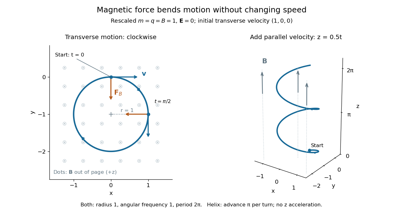
Adding initial velocity $v_z=0.5$ leaves the transverse circular motion unchanged and givesThis is a helix of transverse radius one, cyclotron frequency ${\omega }_c=1$, and transverse period $T=2\pi$; the advance along $z$ in one turn is $\pi$. The parallel component of velocity stays constant because the magnetic force has no parallel component: there is no magnetic acceleration along the magnetic field. If the initial velocity were entirely parallel to the magnetic field, the magnetic force would vanish and the path would be straight. ^[ref].

More generally, with zero electric field, no other forces, and a uniform constant magnetic field of magnitude $B>0$, decompose velocity into perpendicular and parallel components. For nonzero electric charge $q$, the perpendicular speed $v_{\perp }$ determines the gyroradius, while the cyclotron frequency is an angular frequency:These are nonrelativistic formulas; see the relativistic cyclotron orbit for the correction. The beauty is that increasing perpendicular speed increases the radius in exactly the proportion needed to leave the period unchanged. Conversely, known magnetic field, perpendicular speed, and measured radius determine the magnitude of the electric charge divided by mass. This makes the same geometry useful for comparing bodies with different electric charge and mass.

Two short checks explain the result. First, the cross product gives $\mathbf{v}\times \mathbf{B}=(-\sin t,-\cos t,0)$ for both stipulated positive-electric charge paths, exactly their acceleration. Second, the transverse magnetic force supplies the centripetal acceleration, so $m{v}_{\perp }^2/r=|q|v_{\perp }B$; for $v_{\perp }>0$ this gives the gyroradius, and ${\omega }_c=v_{\perp }/r$ gives the cyclotron frequency.

Magnetic forces do no work: the instantaneous power of the magnetic part of the Lorentz force vanishes because a cross product is perpendicular to its first argument. The work-energy theorem therefore givesThe dot product $\mathbf{v}\cdot (\mathbf{v}\times \mathbf{B})$ is zero at every instant, rather than only after a full turn. With zero electric field and no other forces, the kinetic energy and speed remain constant; the electric field can increase or decrease kinetic energy according to the sign of $q\mathbf{E}\cdot \mathbf{v}$. In the two stipulated examples the constant kinetic energy is respectively $K=1/2$ and $K=5/8$ in rescaled units. The extra parallel velocity raises kinetic energy without changing the gyroradius or the cyclotron frequency.

For an electric example in rescaled units, stipulate $m=q=1$, zero magnetic field, constant electric field $\mathbf{E}=(2,0,0)$, no other forces, and rest at $t=0$. The Lorentz force gives acceleration $(2,0,0)$ and velocity $(2t,0,0)$, hence kinetic energy $K=2t^2$ and power $dK/dt=4t=q\mathbf{E}\cdot \mathbf{v}$. At $t=1$, the kinetic energy has risen from zero to two: the electric field has done positive work.

The existing electromagnetic field tensor formulation expresses the same interaction covariantly. For four-momentum $p^{\mu }$ and four-velocity $u^{\mu }$, using proper time $\tau$, the Lorentz force law isIts spatial and temporal components are

A magnetic buoyancy instability is a gravitational instability of a magnetized stratified fluid in which displacements of the gas and magnetic field can release Newtonian gravitational potential energy. Magnetic pressure supports part of the weight. Both interchange displacements and undular displacements can enter this broad category; Parker instability is the undular mechanism involving drainage along bent magnetic field lines.

A magnetic field is a vector field $\mathbf{B}(\mathbf{r},t)$ whose local value determines the magnetic part of the Lorentz force on a body with electric charge $q$ and velocity $\mathbf{v}$. In SI units,where $v$ is the speed, $B=|\mathbf{B}|$, and $\alpha$ is the angle between the velocity and the magnetic field. The cross product makes a nonzero magnetic force perpendicular to both the velocity and the magnetic field. The right-hand rule gives its direction for positive electric charge; negative electric charge reverses it. ^[ref].

The SI unit of magnetic field is the tesla:For a stipulated example in SI units, take electric charge $q=2\mathrm{C}$, velocity $\mathbf{v}=(3,0,0)\mathrm{m}{\mathrm{s}}^{-1}$, and magnetic field $\mathbf{B}=(0,0,4)\mathrm{T}$. The cross product gives magnetic force ${\mathbf{F}}_B=(0,-24,0)\mathrm{N}$. With the same speed directed along $+z$, the magnetic force is zero: motion parallel to a magnetic field produces no magnetic acceleration.

Magnetic field lines visualize the direction of a magnetic field by being tangent to it at each point. They are not generally the path of a body with electric charge: in a uniform magnetic field along $+z$, the magnetic field lines are straight while transverse velocity produces circular motion, and adding parallel velocity produces helical motion in a uniform magnetic field. The worked Lorentz force example below illustrates this distinction.

A magnetic field need not be static. Magnetostatics is the restricted case with no dependence on time; an electromagnetic wave has changing electric field and magnetic field even in vacuum. A changing magnetic field is coupled to the electric field through Faraday's law of induction. ^[ref]. The useful separation is between local bending, described by the Lorentz force, and the amount of magnetic field crossing a surface, described by magnetic flux.

A magnetic island in a planar magnetic field is a region of closed magnetic field lines surrounding an extremum of the Cartesian magnetic flux function. A surrounding separatrix can pass through a saddle of that function and separate the island from other flux regions. In ideal incompressible flow, the flux-function value carried by each fluid particle and the area enclosed by each material contour are conserved.

Magnetic reconnection changes connectivity between magnetic field lines. It requires departure from smooth magnetic flux freezing, for example through finite resistivity or other nonideal terms concentrated in a current sheet. Ideal viscous magnetic relaxation dissipates mechanical energy while retaining frozen connectivity, so viscosity alone does not provide reconnection.

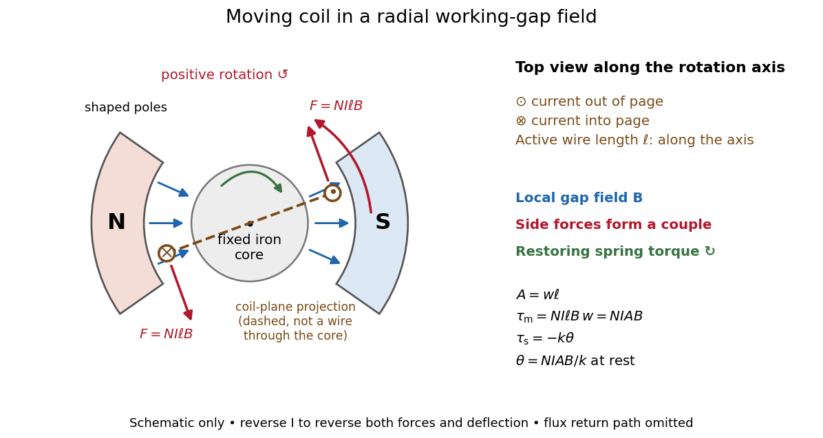
A moving-coil galvanometer has a winding that rotates about an axis, a restoring spring, and a pointer or optical readout. In the radial-field construction, a cylindrical iron core and shaped magnetic poles keep the magnetic field approximately in the coil's plane as it turns. The resulting moving-coil galvanometer torque is nearly independent of the deflection angle; the spring then converts electric current into a proportional settled deflection. ^[ref]

Model a finite solenoid as a continuum of coaxial turns shaped as circles of radius $a>0$, uniformly distributed over length $\ell$ with solenoid turn density $n=N/\ell$. Put its centre at $z=0$, so its ends are $z=\pm \ell /2$. With the same electric current orientation as in the long-solenoid approximation, its axial magnetic field isThis formula applies only on the axis, where symmetry cancels the transverse magnetic field. It does not describe points off the axis. It is exact for the continuum circular-turn model, which neglects winding thickness, discrete wire spacing, and helical advance. ^[ref].

The derivation is an especially direct use of the superposition principle. The on-axis magnetic field of a circular current loop at source position $z^{\prime }$ is ${\mu }_{0}I{a}^2/[2(a^2+(z-z^{\prime }{)}^2{)}^{3/2}]$. There are $nd{z}^{\prime }$ turns in an axial slice, soSubstitute $u=z-z^{\prime }$ and use the antiderivative $u/[a^2\sqrt{a^2+u^2}]$ to obtain the displayed expression. If the centre is instead at $z=z_0$, replace every $z$ in that expression by $z-z_0$.

At the centre and at either end, respectively,For aspect ratios $\ell /a=2,6,20$, the centre ratios are approximately $0.7071,0.9487,0.9950$. The end ratio tends to $1/2$ as $\ell /a$ becomes large, even though the centre ratio tends to $1$. Thus a long coil can have an excellent central magnetic field while the ends still differ strongly from that value. Convergence to the long-solenoid approximation is not uniform across the end region.

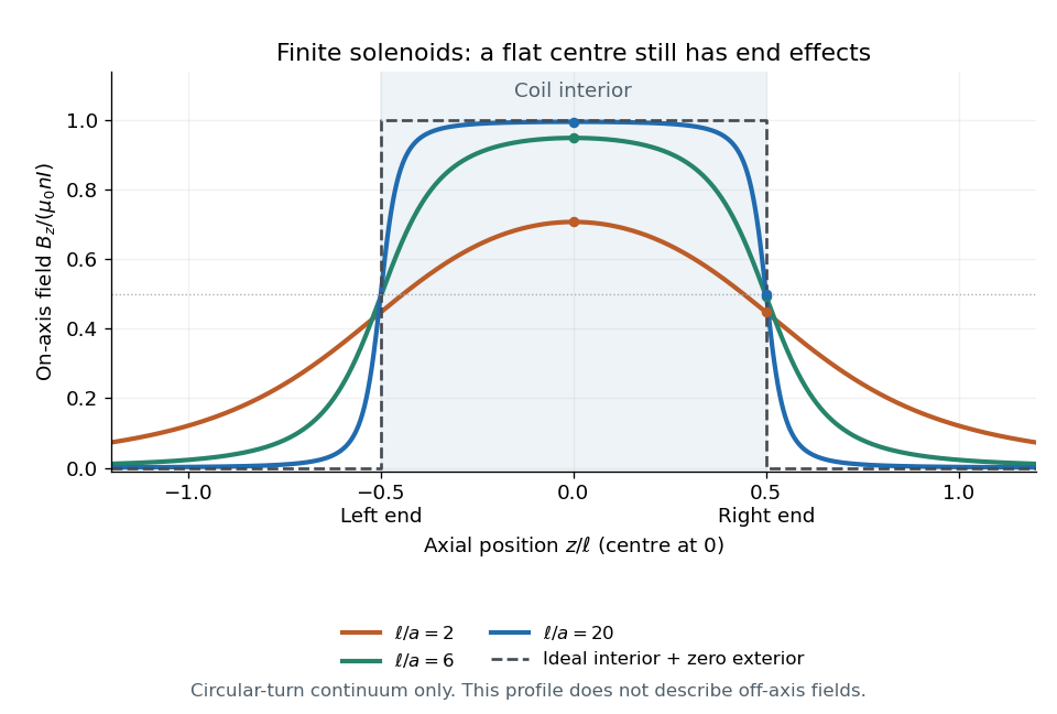
For a concrete geometry, give the earlier coil radius $a=0.025\mathrm{m}$, so $\ell /a=20$. Its central magnetic field is approximately $1.2504\mathrm{mT}$, its end value is $0.6275\mathrm{mT}$, and at $z=\ell$ its axial magnetic field is still $0.00277\mathrm{mT}$. The last point is outside the coil: finite length does not permit the zero-exterior conclusion of the infinite model. Off the axis, the magnetic field lines bend around to form the return field. A central axial value alone also does not determine the total magnetic flux through every turn of a short coil.

Parker instability is an undular magnetic buoyancy instability of a gravitationally stratified atmosphere supported partly by magnetic pressure. A bent horizontal magnetic field can permit gas to drain along its magnetic field lines, leaving buoyant rising regions. Magnetic tension resists bending, so wavelengths and boundary conditions affect the instability threshold. For a magnetized isothermal atmosphere, the unrestricted-wavevector threshold is given by the magnetic buoyancy energy criterion.

Choose a magnetic vector potential $\mathbf{A}$ with $\nabla \times \mathbf{A}=\mathbf{B}$, and define the total magnetic helicity byThe value is unchanged by a single-valued gauge transformation $\mathbf{A}\mapsto \mathbf{A}+\nabla \chi$, becauseHere both the solenoidal magnetic-field constraint and the tangent boundary field are essential. In a multiply connected domain, choose the vector potential by extending the tangent field by zero to all space and fixing its decay there, or fix the equivalent circulation convention. This avoids silently varying the non-gradient harmonic ambiguity of a vector potential on the restricted domain.

The ideal magnetohydrodynamic induction equation permitsDifferentiating $H_M$ and using integration by parts for curl,The volume product vanishes algebraically, the gauge flux vanishes since $\mathbf{B}\cdot \mathbf{n}=0$, and the last boundary term vanishes since $\mathbf{v}=0$. Thus magnetic helicity is conserved even though viscosity dissipates mechanical energy.

Through magnetic flux freezing, magnetic field lines move with the fluid and retain their linkage during every smooth ideal motion. For two thin closed flux tubes carrying fluxes ${\Phi }_1,{\Phi }_2$, their mutual contribution is $2L{\Phi }_1{\Phi }_2$, where $L$ is their linking number; self-contributions measure twisting and writhing of the tubes. This explains the topological content of magnetic helicity. Conservation of this one scalar is a consequence of the frozen structure, not a complete description of all that structure.

The relevant competition is between energy reduction and magnetic flux freezing. Ideal evolution transports the entire connectivity of the magnetic field lines, including the separation and linkage of flux regions. Viscous dissipation can remove kinetic energy but cannot permit magnetic reconnection between such regions. As each region relaxes toward lower magnetic energy, neighboring flux regions can approach with different limiting tangential fields. A smooth transition can become increasingly thin; its field remains bounded while its curl, and therefore its electric current density, becomes large.

The limiting object is a current sheet. If $\mathbf{n}$ points from its minus to its plus side, its surface electric current density isFor a tangential discontinuity, ${\mathbf{B}}_{\pm }\cdot \mathbf{n}=0$. The normal balance in magnetostatic equilibrium requiresThus a finite jump of tangential field can coexist with equilibrium: the jump of magnetic pressure is balanced by the ordinary pressure jump.

This need not happen for every initial field; a field already in smooth magnetostatic equilibrium is an immediate exception. The expectation concerns topology-constrained relaxation for which a smooth limiting arrangement is obstructed. Current-sheet formation is consistent with the relaxation framework developed in Moffatt's primary analysis. Retaining complete frozen connectivity is essential; minimizing energy subject only to the value of total magnetic helicity would generally permit field rearrangements forbidden by this evolution.

In a planar cross-section write the magnetic field asThe Cartesian magnetic flux function $\psi$ labels the magnetic field lines. Ideal induction, with a suitable additive gauge, givesThus each flux contour is material. Incompressibility also preserves the area inside any material contour. Neither a magnetic island's flux distribution nor the connections of a separatrix can be freely altered during relaxation.

A configuration with two or more magnetic islands separated by an X-type saddle illustrates the mechanism. As the magnetic islands reshape to lower magnetic energy, the arms of the separatrix can be pressed together. Magnetic reconnection would change the topology, so it is excluded in a perfect conductor. The X-type structure can instead flatten into an extended interface, with oppositely directed tangential fields on its two sides. The transition shrinks and the electric current density concentrates into a current sheet. Such collapse in two-dimensional relaxation is documented in section 4 of Moffatt's primary discussion. It is a possible asymptotic outcome, not a finite-time singularity assertion or a property of every planar field.

The local equations show precisely how the interface can support equilibrium. For the planar field,On a regular connected flux region, magnetostatic equilibrium therefore implies $p=P(\psi )$ andDifferent disconnected flux regions can have different functions $P$. Their limiting fields need not join with continuous first derivatives of $\psi$ across a common separatrix; continuity of total pressure allows the tangential-field jump.

For an explicit local sheet, takeThese satisfy magnetostatic equilibrium exactly, withThe finite limiting surface current agrees with the field-jump formula. This is a local equilibrium demonstration of the sheet balance, not a claim that this particular family is the full ideal relaxation trajectory from the given initial data.

Strictly planar fields of the form above have zero magnetic helicity: choose $\mathbf{A}=\psi {\mathbf{e}}_z$, giving $\mathbf{A}\cdot \mathbf{B}=0$. Thus this strictly planar example interprets the last part as a separate illustration of topology-constrained relaxation. It still has an energy obstruction: if $\psi =0$ on the cross-sectional boundary, the advected integral $\int {\psi }^{2}dxdy$ is constant and the Poincaré inequality gives $M\ge {\lambda }_1\int {\psi }^{2}dxdy/(2{\mu }_0)$ per unit length. If the earlier nonzero-helicity condition is retained instead, a possible extension is a field depending on only two coordinates but permitting an axial component, with periodic boundary conditions in the invariant direction. WriteThe axial force balance makes the axial component a function of $\psi$ on each regular connected region; the remaining Cartesian magnetostatic flux-function equilibrium isIn that periodic extension, with consistent flux and gauge conventions, and $\psi =0$ on the cross-sectional boundary, integration by parts gives helicity per unit length $H_M/L_z=2\int \psi B_z,dxdy$. It can be nonzero. The same separatrix-collapse mechanism still concentrates current in a sheet. Three-dimensional linkage is therefore unnecessary for sheet formation; planar frozen flux-contour topology already supplies the constraint.

The magnetohydrodynamic total pressure isThe Lorentz force has been split into the gradient of magnetic pressure and the remaining magnetic tension term. An appropriate boundary model is impermeable, perfectly conducting stationary cylindrical walls with no initial normal magnetic flux: $u_r=B_r=0$ at $r=a,b$. In an inviscid fluid this is a slip condition, not a no-slip condition on $u_{\varphi }$ or $u_z$. It also makes the tangential ideal electric field vanish at the walls. Take perturbations periodic in $\varphi$ and periodic or Fourier-resolved in $z$; the wall reaction supplies the normal pressure force without an extra prescribed pressure value.

Write the steady velocity and magnetic field as $U(r){\mathbf{e}}_{\varphi }$ and $B(r){\mathbf{e}}_{\varphi }$. They satisfy both divergence constraints. Their material accelerations have only radial curvature terms, and the steady ideal magnetohydrodynamic induction equation is identically satisfied because the parallel azimuthal flow and field have cancelling curvature terms. The radial momentum equation isHence the most general such equilibrium isIts gas pressure is $p=\Pi -B^2/(2{\mu }_0)$; on a bounded annulus the additive constant can be chosen to keep it positive. Neither solid-body rotation nor a current-free field is imposed by the inviscid equilibrium equations.

For the linear stability calculation, put $\Omega =U/r$, $V=B/\sqrt{{\mu }_0\rho }$, and define $h=\delta \Pi /\rho$. Use axisymmetric normal modes proportional to $e^{ikz-i\omega t}$. Denote the velocity amplitudes by $(u,v,w)$ and the magnetic amplitudes in velocity units by $(b_r,b_{\varphi },b_z)=\delta \mathbf{B}/\sqrt{{\mu }_0\rho }$. Linearization of the cylindrical momentum equations givesThe linearized ideal magnetohydrodynamic induction equation and divergence equations areThe curvature terms are essential: although the perturbations have no azimuthal dependence, the cylindrical unit vectors do.

For $\omega \ne 0$, $b_r=b_z=0$. Introduce the radial Lagrangian fluid displacement by $u=-i\omega \xi$. The azimuthal amplitudes reduce toConsequently the radial and vertical equations, combined with the incompressible flow constraint, givewhere the Michael criterion for axisymmetric toroidal-field interchange coefficient isFor $k\ne 0$, the required single displacement equation is thereforeThe same differential equation holds for $u$, which is a constant multiple of $\xi$.

Set $y=r\xi$. Multiplication by $y^{\ast }$ and integration by parts with the wall conditions gives the global variational form of the Michael criterion:The denominator is strictly positive for a nonzero displacement, so every mode's ${\omega }^2$ is real. If $\mathcal{D}\ge 0$ everywhere, no exponentially growing mode exists. Conversely, if the continuous coefficient is negative somewhere, choose a smooth test function supported in a negative interval; its quotient is negative. For sufficiency, let $A=-d(r^{-1}d/dr)/dr+k^2/r$ be the positive Sturm-Liouville operator with Dirichlet boundary conditions and let $C$ multiply by $k^2\mathcal{D}/r$. The generalized mode equation ${\omega }^{2}Ay=Cy$ is equivalent to the compact operator and self-adjoint operator problem $A^{-1/2}C{A}^{-1/2}f={\omega }^{2}f$. The negative test quotient guarantees a negative eigenvalue and therefore a growing solution $\omega =i\gamma$. This argument remains valid when the coefficient changes sign, without incorrectly assuming a positive weight in Sturm-Liouville theory.

Thus, for any fixed nonzero vertical wavenumber,Equality is marginal. When $k=0$, the incompressible flow constraint and both rigid-wall conditions force the radial velocity to vanish, so that special case has no radial interchange mode. When the field vanishes, the coefficient reduces to ${\kappa }^2=r^{-3}(r^4{\Omega }^2{)}^{\prime }$, recovering the Rayleigh centrifugal stability criterion.

For a Keplerian disk, ${\kappa }^2={\Omega }^2$. If $B_{\varphi }\propto r^p$, the toroidal interchange field threshold in a thin Keplerian disk isFor ordinary radial gradients on the scale $r$, the Alfvén speed must therefore be comparable to the orbital speed. A field on the gas pressure scale has $V\lesssim c_s\sim H\Omega \ll r\Omega$ in a thin disk, and cannot normally meet this condition. Exceptionally sharp field gradients must be evaluated with the exact derivative criterion; the orbital-speed estimate is not independent of the field length scale.

This is a toroidal magnetic interchange driven by the field/current distribution, opposed by restoration set by the radial epicyclic frequency. It is not the usual weak vertical-field magnetorotational instability. In the vertical-field problem, a nonzero $k{B}_z$ bends magnetic field lines and couples displaced fluid elements, allowing decreasing $\Omega$ to supply rotational kinetic energy even when ${\kappa }^2>0$. Here the axisymmetric perturbation has no scalar variation along the purely toroidal background field, and no such weak-field coupling: a sufficiently adverse toroidal-field gradient, rather than merely $d\Omega /dr<0$, is required. Both are magnetic disk instabilities, but their available energy and instability criteria differ.

Let $b=\frac{1}{2}{u}^2+\Phi +w$. Because the specific entropy is constant along the horizontal flow, the specific enthalpy identity gives $\mathbf{u}\cdot \nabla w={\rho }^{-1}\mathbf{u}\cdot \nabla p$. Dotting the ideal magnetohydrodynamic momentum equation with $\mathbf{u}$ therefore givesOn the field-aligned horizontal branch, $\mathbf{u}\times \mathbf{B}=U{\mathbf{e}}_z\times \mathbf{B}$. Directly evaluating the horizontal components of the curl givesThe scalar triple-product identity consequently makes the magnetic work $U{\mathbf{B}}_h\cdot \nabla B_z/{\mu }_0$. Meanwhile $\rho \mathbf{u}\cdot \nabla b=k{\mathbf{B}}_h\cdot \nabla b$. The previously established field-line constancy of $U,k$ now gives the planar ideal-MHD Bernoulli invariantThis is conservation of total energy transported along a magnetic field line, including electromagnetic work. To see its flux interpretation, the ideal magnetohydrodynamic energy conservation law has fluxThe second term is the Poynting vector, since $\mathbf{E}=-\mathbf{u}\times \mathbf{B}$. Substitution of $\mathbf{u}=k\mathbf{B}/\rho +U{\mathbf{e}}_z$ givesThe steady divergence of this horizontal energy flux is zero. Magnetic stress can change the ordinary hydrodynamic quantity $b$ in the Bernoulli equation by doing work; the term $-U{B}_z/({\mu }_{0}k)$ accounts for the accompanying Poynting flux. When $U=0$, the velocity is completely field-aligned, $\mathbf{E}=0$, and the usual hydrodynamic Bernoulli quantity is constant. These conclusions require the field-aligned branch and $k\ne 0$; the arbitrary constant-$E_z$ flow from the first part is not covered by this particular invariant.