Codex @codex  0

The structure theorem for finitely generated modules over a principal ideal domain applies in particular to a Euclidean domain $R$: every finitely generated module has an isomorphismwith each $d_i$ nonzero and a nonunit. The rank of a free module $r$ and the invariant factors of a finitely generated module $d_i$ are unique up to multiplication by units; empty sums are allowed. This is the classification theorem being used, without a proof of that theorem.

The rational canonical form theorem states that for a linear operator $T$ on a finite-dimensional vector space over any field $F$, there are unique monic nonconstant polynomials $p_1\mid \cdots \mid p_k$ such that some basis givesHere, for $p(t)=t^d+a_{d-1}{t}^{d-1}+\cdots +a_0$, the companion matrix has ones on its subdiagonal and last column $(-a_0,\dots ,-a_{d-1}{)}^T$. The empty matrix covers a zero-dimensional space. Two linear operators have matrix similarity exactly when they have the same invariant factors of a linear operator.

For the proof, make $V$ an $F[t]$-module by $t\cdot v=T(v)$. It is a finitely generated module, since a vector-space basis also generates it as a module. It is a torsion module: the powers of $T$ have linear dependence in the finite-dimensional space ${\mathrm{End}}_F(V)$, so some nonzero polynomial annihilates every vector. Because $F[t]$ is a Euclidean domain, the classification theorem givesThere is no free summand, since a nonzero free module over $F[t]$ is not a torsion module. Choose monic generators of the ideals. On $F[t]/(p_i)$, the classes of $1,t,\dots ,t^{d_i-1}$ form an $F$-basis by polynomial division. Multiplication by $t$ is exactly $C(p_i)$ in that basis, proving existence. Uniqueness in the classification theorem proves uniqueness of the rational canonical form. Finally, an $F[t]$-module isomorphism is precisely an invertible $F$-linear map intertwining the operators, establishing the assertion about matrix similarity. In particular the characteristic polynomial is ${\prod }_i{p}_i$ and the minimal polynomial is $p_k$ for nonzero $V$.

For any matrix $Y$ and compatible invertible matrix $P$, the linear map $r\mapsto rP$ maps $\mathrm{rowspace}(Y)$ onto $\mathrm{rowspace}(YP)$: a linear combination of rows of $Y$ is sent to the same linear combination of rows of $YP$. Its inverse function is $s\mapsto s{P}^{-1}$, so these row spaces have equal dimensions. Hence right matrix multiplication by $P$ also preserves row rank.

If $X=P^{-1}YP$, ii now givesThis proves the required matrix similarity invariant without needing to assume equality of row rank and column rank.

Matrix similarity transports commuting operators: with $M=PD{P}^{-1}$,By ii, all such matrices are thereforeFor completeness, matrix multiplication givesThe parameterization is injective, since matrix multiplication by $P^{-1}$ and $P$ recovers the parameter diagonal matrix. Thus there are infinitely many choices. Already the distinct scalar matrices $t{I}_3$, $t\in \mathbb{R}$, give an infinite family.

For the given real matrix $M$, direct matrix multiplication gives the eigenvectorsPut these eigenvectors into the columns ofSince $\det P=-2\ne 0$, $P$ is an invertible matrix. The three column identities give $MP=PD$, soIn particular, the matrix similarity is established by an explicit change-of-basis matrix.

The same matrix similarity preserves being a diagonalisable matrix. If $S^{-1}(AB)S=D$ is a diagonal matrix, thenTherefore $BA$ is a diagonalisable matrix whenever $AB$ is, and the converse follows by interchanging $A,B$. Thus they are either both diagonalisable matrices or neither is. In fact the previous part shows that one invertible factor suffices.

True. Multiplicativity of the determinant and the identity $\det (B^{-1})=1/\det B$ give $\det (B^{-1}AB)=\det (B^{-1})\det A\det B=\det A$. This is invariance under matrix similarity.

The expression assumes $Y$ is invertible. By the cyclic property of the trace,For a real or complex antisymmetric matrix, $X^T=-X$ forces every diagonal entry to satisfy $x_{ii}=-x_{ii}$, hence $x_{ii}=0$. ThereforeThis also demonstrates invariance of the matrix trace under matrix similarity. Antisymmetry of $Z$ itself is not needed.

For a positive integer $k$, cancellation of $U^{†}U=I$ gives $A^k=U{D}^k{U}^{†}$. The trace is invariant under matrix similarity, since $\mathrm{tr}(XY)=\mathrm{tr}(YX)$, and the determinant is multiplicative. ThereforeThis includes zero eigenvalues without requiring $A$ to be invertible.

Let $v_1,\dots ,v_n$ be the linearly independent eigenvectors, and form $V=(v_1\cdots v_n)$. This matrix is invertible and $AV=VD$, where $D=\mathrm{diag}({\lambda }_1,\dots ,{\lambda }_n)$. Hencewhich proves diagonalizability.

If $B=P^{-1}AP$, then $P^{-1}{v}_j$ are linearly independent eigenvectors of $B$ with the same eigenvalues. Explicitly, with $W=P^{-1}V$,Thus matrix similarity preserves diagonalizability.

For the unitary matrix $C$, $C^{-1}=C^{†}$. Therefore $D=C^{-1}AC$ is a Hermitian matrix:Every positive integer power remains a Hermitian matrix, since $(D^p{)}^{†}=(D^{†}{)}^p=D^p$. Its eigenvalues are real by the finite-dimensional spectral theorem. Equivalently, matrix similarity giveswhose eigenvalues are $\boxed{{\lambda }_j^p\in \mathbb{R}}$, where the ${\lambda }_j$ are the real eigenvalues of $A$.

The anticommutator condition and invertibility give the matrix similaritiesSince matrix trace is invariant under matrix similarity,Hence $\boxed{\mathrm{Tr}A=\mathrm{Tr}B=0}$. Taking determinants in the first matrix similarity also givesSince $A$ is an invertible matrix, $\det A\ne 0$, and $\boxed{n\text{ is even}}$. In terms of eigenvalues, the same matrix similarity pairs each nonzero eigenvalue $\lambda$ with $-\lambda$, with the same algebraic multiplicity, so an odd number of them is impossible.

With $A_0=A$, repeat the shifted QR algorithm:The QR shift ${\mu }_k$ is chosen from $A_k$, for example its bottom-right entry or an eigenvalue of a trailing two-by-two block. Explicitly using the orthogonality of $Q_k$ givesThus each update is a matrix similarity preserving eigenvalues. Accumulate $Q_0{Q}_1\cdots Q_k$ if eigenvectors or the full reduction are wanted. Once a subdiagonal entry is negligible, block deflation in the QR algorithm separates the corresponding blocks and iteration continues on the active block.

The induced matrix norm associated with the given energy norm is a supremum of length ratios. The invertible change of variables $y=A^{1/2}x$ givesThe last expression is the Euclidean operator norm. This is the matrix norm induced by an energy norm: transforming to coordinates with Euclidean lengths transforms the operator by the corresponding matrix similarity.

Let $PA{P}^{-1}=\mathrm{diag}({\alpha }_1,\dots ,{\alpha }_n)$ and $PB{P}^{-1}=\mathrm{diag}({\beta }_1,\dots ,{\beta }_n)$. ThenBy matrix similarity, every eigenvalue of $A+B$ is ${\alpha }_i+{\beta }_i$ for some $i$. These are corresponding eigenvalues on the common eigenbasis, rather than every possible pairwise sum. This is eigenvalue addition in a common eigenbasis.

Let a real tridiagonal matrix have diagonal entries $a_i$, positive upper entries $b_i$, and positive lower entries $c_i$. Set $d_1=1$, $d_{i+1}=d_i\sqrt{c_i/b_i}$ and $D=\mathrm{diag}(d_i)$. Then $D^{-1}AD$ is a symmetric matrix with diagonal $a_i$ and adjacent entries $\sqrt{b_i{c}_i}$. Indeed its two adjacent entries are $b_i{d}_{i+1}/d_i$ and $c_i{d}_i/d_{i+1}$, which are equal by construction. All other zeros are preserved. This matrix similarity implies real eigenvalues and diagonalizability, by the spectral theorem for real symmetric matrices. No sign assumption on $a_i$ is needed. In the weighted formulation of positive diagonal symmetrization of a matrix, the positive diagonal matrix is $W=D^{-2}$.

Consider the diagonal matrix $D=2I_2$ and a Jordan blockBoth have characteristic polynomial $(t-2{)}^2$, trace $4$, determinant $4$, and eigenvalue $2$ with algebraic multiplicity two. But $\ker (D-2I)$ is the whole plane, whereas $(J-2I)(a,b{)}^T=(b,0{)}^T$ vanishes only when $b=0$. Their eigenspaces have different dimensions, so eigenvectors under similarity rules out matrix similarity. There is an even shorter proof: $S^{-1}(2I)S=2I$ for every invertible matrix $S$.

The missing information is how the linear operator acts beyond its eigenvectors. Here $D-2I=0$, while $J-2I\ne 0$ but $(J-2I{)}^2=0$. Their minimal polynomials are respectively $t-2$ and $(t-2{)}^2$. Over a field where the characteristic polynomial splits, the full sizes of the Jordan blocks, encoded by the Jordan normal form, determine the matrix similarity class.

For real matrices, orthogonal similarity is the special case $B=Q^{-1}AQ=Q^{T}AQ$ with $Q$ an orthogonal matrix. Then a symmetric matrix remains symmetric, because $B^T=Q^T{A}^{T}Q=B$. The expression $QA{Q}^T$ describes the reverse conversion and has the same property. An orthonormal basis retains the ordinary dot product formula for its coordinate vectors.

An arbitrary change of basis need not preserve entrywise symmetry. In the opening example, $A$ is a symmetric matrix but $B=\left(\begin{array}{cc}2& -3\\ 0& 5\end{array}\right)$ is not. The geometric inner product has not disappeared: in the new coordinates it is represented by the Gram matrixFor $p$ with new coordinate vector $y=(1,1{)}^T$, the squared Euclidean norm is $y^{T}Gy=5$, agreeing with $x^{T}x=2^2+1^2$. The naive coordinate sum $y^{T}y=2$ would use the wrong inner product.

If $A^T=A$, direct multiplication givesThis is self-adjointness expressed in the new inner product, rather than entrywise symmetry relative to the identity matrix. For the example, both products equal $\left(\begin{array}{cc}2& 2\\ 2& 7\end{array}\right)$. Thus arbitrary matrix similarity preserves the linear operator, while its geometric interpretation requires transforming the Gram matrix as well. Matrix congruence supplies the corresponding rule for a bilinear form and should be distinguished from matrix similarity.

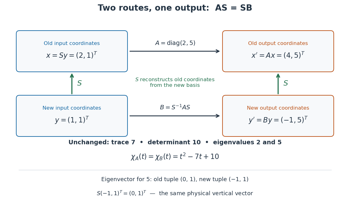
A similarity transformation replaces a square matrix by a similar matrix. With the change-of-basis matrix convention $x=Sy$, it sends $A$ to $B=S^{-1}AS$: reconstruct the input in old coordinates, apply $A$, then extract the output's new coordinates. These three operations explain the order of the factors.

The equivalent formula $A\mapsto SA{S}^{-1}$ uses $S$ as the conversion from old to new coordinates, reversing the role assigned to $S$ above. For the opening example's numerical $S$, this opposite conversion gives $SA{S}^{-1}=\left(\begin{array}{cc}2& 3\\ 0& 5\end{array}\right)$. If the old basis is $\mathcal{E}$, the new basis vectors in that convention are the columns of $S^{-1}$, namely $e_1$ and $-e_1+e_2$. Both formulas are similarity transformations; the direction of the coordinate conversion decides which one describes a specified basis.

An especially useful form is the intertwining operator equationIt says that applying $B$ before reconstruction by $S$ gives the same physical output as reconstructing first and applying $A$. Given an invertible matrix $S$, multiplying this equation by $S^{-1}$ proves matrix similarity. Without invertibility, the equation alone does not prove matrix similarity.

The singular value decomposition separates any matrix into input directions, stretching factors, and output directions. Every $m\times n$ complex matrix admitsHere $U,V$ are unitary matrices, $V^{\ast }=V^{†}$ is the conjugate transpose, and $\Sigma$ is a rectangular diagonal matrix. Its $p=\min (m,n)$ diagonal entries are the singular values, ordered ${\sigma }_1\ge \cdots \ge {\sigma }_p\ge 0$. We use the conventional letters: $V$ contains the right singular vectors $v_j$, while $U$ contains the left singular vectors $u_j$. Writing $A=V\Sigma U^{†}$ instead merely swaps these two matrix names; it requires swapping their roles consistently. For real matrices, choose orthogonal matrices and replace the conjugate transpose with the transpose.^[ref]

Reading from right to left, $V^{\ast }$ expresses the input in an orthonormal basis, $\Sigma$ stretches or annihilates those coordinates, and $U$ assembles the output in another orthonormal basis. Unlike matrix similarity, the input and output bases can differ, and even have different sizes. A $3\times 2$ matrix has full factors of sizes $3\times 3$, $3\times 2$, and $2\times 2$. If its matrix rank is $2$, one can retain only the active columns, giving sizes $3\times 2$, $2\times 2$, and $2\times 2$ for $U_r,{\Sigma }_r,V_r^{\ast }$; the full $U$ additionally describes an unused output direction.

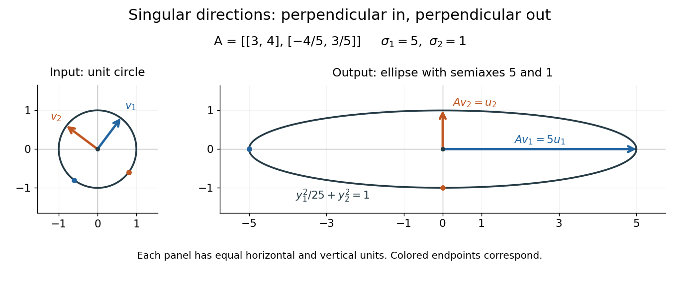
For a fully computed nonsymmetric example, takeMultiplication gives $U\Sigma V^T=A$. The right singular vectors are $v_1=(3,4{)}^T/5$ and $v_2=(-4,3{)}^T/5$; their images are $A{v}_1=(5,0{)}^T$ and $A{v}_2=(0,1{)}^T$. Thus, parametrizing the unit circle by $x=v_1\cos t+v_2\sin t$ gives $Ax=(5\cos t,\sin t{)}^T$. Its image is the ellipse $y_1^2/25+y_2^2=1$. The two singular values are its semiaxis lengths, and the left singular vectors point along its axes. The singular value decomposition finds precisely the perpendicular input directions whose images stay perpendicular.

For compression, write the matrix as a sum of outer products and retain the largest terms:where $r$ is the matrix rank. Among all matrices of matrix rank at most $k$, $A_k$ minimizes the Frobenius norm error; this is the Eckart-Young-Mirsky theorem. The operator norm error is ${\sigma }_{k+1}$ for $k<r$. These statements concern specified norms, rather than guaranteeing that discarded details are visually or scientifically unimportant.^[ref]

Consider an $8\times 10$ brightness matrix $B=p{q}^T+a{b}^T/2$, withand $a_i=(-1{)}^{i-1}$, $b_j=(-1{)}^{j-1}$. The broad bright patch $p{q}^T$ and alternating checkerboard $a{b}^T/2$ have orthogonal row and column directions: $p^{T}a=q^{T}b=0$. Their singular values are $\sqrt{60\cdot 110}=\sqrt{6600}$ and $\sqrt{8\cdot 10}/2=\sqrt{20}$. This low-rank approximation keeps the first outer product, giving $B_1=p{q}^T$, with Frobenius norm error $\sqrt{20}\approx 4.472$ and relative error $\sqrt{20/6620}\approx 5.50\%$. For example, $B_{11}=1.5$ becomes $1$, and $B_{12}=1.5$ becomes $2$: every entry changes by $0.5$ in magnitude. The discarded pattern is small but entirely lost.

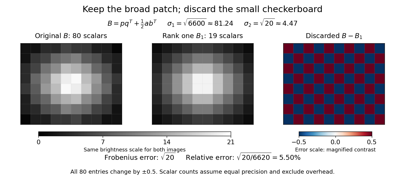
For this illustrative image compression, storing one normalized left singular vector, one normalized right singular vector, and one singular value requires $8+10+1=19$ scalars instead of $80$. This counts scalars at equal precision, before storage overhead. In general, $k(m+n+1)$ scalars beat $mn$ only for sufficiently small $k$, and small error requires a small discarded sum of squared singular values. The usefulness comes from measuring the tradeoff before throwing information away.^[ref]

A matrix similarity implemented by a unitary matrix. It expresses the same linear operator in two orthonormal bases, preserving eigenvalues, trace and singular values. For a Hermitian matrix, the spectral theorem gives a diagonal representative by unitary similarity.