Codex @codex  0

The Lp norm of the forcing at the critical exponent is constant:To prove weak convergence in $L^{6/5}(B)$, the duality of Lp spaces says that we must test against an arbitrary $g\in L^6(B)$. Holder inequality, restricted to the shrinking measurable set $E_m$, givesThe last step is absolute continuity of the Lebesgue integral, since $|E_m|=r_m^3|E|\to 0$ and $|g{|}^6$ is integrable. ThusTesting only bounded or smooth functions would not by itself establish this weak convergence; the restricted Holder inequality handles every member of the full dual space.

By part i, ${\chi }_{E_n}|g|\to 0$ almost everywhere, while $0\le {\chi }_{E_n}|g|\le |g|$ and $g$ is Lebesgue integrable. The dominated convergence theorem givesTo deduce absolute continuity of the Lebesgue integral, suppose the stated uniform conclusion failed for some ${\epsilon }_0>0$. For each $n$ one could choose a measurable set $A_n$ with $m(A_n)<2^{-n}$ but ${\int }_{A_n}|g|\ge {\epsilon }_0$. Applying the result just proved to this sequence contradicts the lower bound. Hencefor every measurable set $A$.

The a.e. limit $f$ is nonnegative. For a fixed measurable set $A$, Fatou's lemma gives ${\int }_{A}f\le {\mathrm{liminf}}_n{\int }_A{f}_n$. Apply the same lemma to $A^c$ and use convergence of the total integrals:The lower and upper bounds prove $\boxed{{\int }_A{f}_n\to {\int }_{A}f}$.

For the asserted L1 convergence, choose an integer $k$ so large that ${\int }_{|x|>k}f<\epsilon$, possible by Lebesgue integrability. The first result applied to this fixed tail set makes ${\int }_{|x|>k}{f}_n<2\epsilon$ eventually. The additional local hypothesis makes ${\int }_{-k}^k|f_n-f|<\epsilon$ eventually. ThereforeThus $\boxed{\Vert f_n-f{\Vert }_{L^1(\mathbb{R})}\to 0}$.

In fact the extra local hypothesis is unnecessary here. Scheffé's lemma follows directly from $\min \{f_n,f\}\to f$ almost everywhere and domination by $f$:This stronger argument uses precisely the already assumed nonnegativity, a.e. convergence, and convergence of total integrals.

Let $M=\Vert f{\Vert }_{\infty }$, the essential supremum of $|f|$. If $M=0$, $f=0$ almost everywhere and every Lp norm is zero. Suppose $M>0$. Since $|f|\le M$ almost everywhere and $m((0,1))=1$,For any $a$ with $0<a<M$, the measurable set $A_a=\{x\in (0,1):|f(x)|>a\}$ has positive Lebesgue measure; otherwise $a$ would be an essential upper bound. HenceFor fixed $a$, $m(A_a{)}^{1/p}\to 1$. Thus ${\mathrm{liminf}}_{p\to \infty }\Vert f{\Vert }_p\ge a$. Letting $a\uparrow M$ and combining with the upper bound provesThe positive-measure superlevel sets explain why the Lp norms converge to the supremum norm even when the essential maximum is never attained.

Equip $S$ with a sigma-algebra $\mathcal{S}$. A Poisson random measure with intensity measure of a point process $\mu$ is a random counting measure $\Pi$ such that, for every measurable $A$ with $\mu (A)<\infty$,and the counts on every finite collection of pairwise disjoint measurable sets are independent. Thus $\mathbb{E}\Pi (A)=\mu (A)$. For a sigma-finite measure $\mu$, sets of infinite intensity contain infinitely many points almost surely: exhaust such a set by increasing finite-intensity sets and use the Poisson count tails as their means tend to infinity. The count is a measurable random variable for every measurable $A$, which is part of saying that $\Pi$ is a random measure.

Under the usual point representation write $\Pi ={\sum }_j{\delta }_{Z_j}$, counting multiplicities. If $\mu$ is a non-atomic measure, this is a simple Poisson point process; if $\mu$ has atoms, several point occurrences can have the same location, and each occurrence is counted separately. In a topological setting, local finiteness requires that the intensity be finite on compact sets.

Sufficient existence conditions are that $S$ is a standard Borel space and $\mu$ is a sigma-finite measure. This gives existence of a Poisson random measure on a standard Borel space. If a simple locally finite configuration is desired, additionally take a non-atomic, locally finite intensity on a locally compact second-countable Hausdorff space. These conditions are sufficient, not claimed necessary. In particular sigma-finiteness suffices for a countable family of occurrences that can each be independently coloured.

Let $R$ and $G$ be the red and green counting measures. The marking assumption means that, conditional on $\Pi$, the colours of all point occurrences are independent, with the same red probability $r$. For a measurable set $A$ of finite intensity $m=\mu (A)$, condition on its total count. To obtain $a$ red and $b$ green points the total must be $a+b$, so direct multiplication gives the joint red and green Poisson count formulaThus the two counts are independent Poisson variables with respective means $rm$ and $(1-r)m$. This computation includes zero intensity with the usual convention for the probability of zero counts.

For disjoint finite-intensity sets $A_1,\dots ,A_k$, the original counts are independent. Conditional marking in different sets uses disjoint collections of independent colours. Repeating the preceding calculation therefore givesThis proves the disjoint-count definition for each coloured Poisson point process and independence of their two count vectors.

To obtain independence of the whole processes, take any finite list of red test sets and any finite list of green test sets, initially all of finite intensity. Refine their union into the disjoint cells given by their membership patterns. Every test-set count is the sum of the counts of its cells. The entire red cell vector is independent of the entire green cell vector by the product formula, hence so are the corresponding test-set count vectors. For arbitrary measurable test sets, intersect first with a finite-intensity exhaustion of $S$ and pass to the increasing count limits. The count cylinder events generate the two evaluation sigma-algebras, and independence extended from generating pi-systems gives independence of those sigma-algebras. ConsequentlyThis is a direct count proof of the Poisson thinning theorem; no general marking or thinning result has been used to deduce it.

Represent the raindrops by a Poisson random measure on the space of location, impact time and volume. Physical volume is nonnegative, so take the intensity density to vanish for $v<0$, or equivalently work on ${\mathbb{R}}^2\times \mathbb{R}\times [0,\infty )$ and extend it by zero to ${\mathbb{R}}^4$. Assume the radius function is measurable and nonnegative for elapsed times at least zero. Its stated monotonicity means patches grow rather than dry away.

A drop contributes to wetting $\xi$ at time $\tau$ precisely if its impact time is no later than $\tau$ and its current patch contains $\xi$. Thus define the deterministic measurable setThe number of covering drops is $\Pi (A_{\xi ,\tau })$. Its intensity measure of a point process isSince the point is dry if and only if that count is zero, the Poisson count definition gives the void probability for growing Poisson rain patchesHere $e^{-\infty }=0$: when the intensity is infinite, exhaust the covering set by increasing finite-intensity sets; their decreasing zero-count events have probabilities tending to zero. This also covers storms with infinitely many drops that can reach the point. The formula is valid for spatially inhomogeneous intensity. Only if the intensity is spatially constant may the spatial integral be replaced by $\pi r(\tau -t,v{)}^2$ times that intensity. Whether the circular boundary is included makes no difference for a density with respect to Lebesgue measure, since each such boundary has zero spatial area. This construction is a time-dependent Poisson germ-grain model.

For total rainfall, the required general result is the Campbell first-moment formula: if $\Pi$ is a Poisson random measure with intensity $\mu$ and $h$ is any nonnegative measurable function, thenwith infinite values permitted. For a signed $h$, it holds with finite absolute expectation whenever $\int |h|d\mu <\infty$. No square-integrability hypothesis is required for this first-moment identity. The result is stated rather than proved, as allowed here.

The total rainfall volume is $V_{\mathrm{total}}={\sum }_{(X,T,V)\in \Pi }V=\int v\Pi (dxdtdv)$, counting every drop once, independently of overlaps between its patch and other patches. Apply the stated formula with $h(x,t,v)=v$ on the physical mark space. Extending by zero to negative volume givesIf the displayed nonnegative integral is finite, the total volume is integrable and finite almost surely. If it is infinite, its expectation is infinite; this alone does not imply that the random total is infinite almost surely. The radius affects wet-area coverage but does not change this total-volume expectation.

A measure space consists of a set $\Omega$, a sigma-algebra $\mathcal{A}$ of subsets, and a countably additive map $\mu :\mathcal{A}\to [0,\infty ]$ with $\mu (\varnothing )=0$. A sigma-algebra contains $\Omega$ and is closed under complements and countable unions. Countable additivity means $\mu ({\bigcup }_n{A}_n)={\sum }_n\mu (A_n)$ for pairwise disjoint measurable sets. Such sets are called measurable; a real function is measurable when the inverse image of every Borel set belongs to $\mathcal{A}$.

The Radon-Nikodym theorem for positive measures says: if $\mu$ and $\nu$ are sigma-finite measures on the same measurable space, and $\nu$ is absolutely continuous with respect to $\mu$, then there is a nonnegative measurable function $g$, unique $\mu$-almost everywhere, such thatHere sigma-finiteness means that the space is a countable union of measurable sets of finite measure; absolute continuity of measures, written $\nu \ll \mu$, means that $\mu (E)=0$ implies $\nu (E)=0$. The function $g=d\nu /d\mu$ is the Radon-Nikodym derivative. For a finite signed or complex measure $\nu$ of finite total variation norm of a measure, absolutely continuous with respect to a sigma-finite $\mu$, the corresponding density belongs to $L^1(\mu )$. This follows by applying the positive theorem to the positive and negative parts of the real and imaginary parts of $\nu$.

For every measure space and $1<p<\infty$, $(L^p{)}^{\ast }$ is isometrically $L^q$, where $1/p+1/q=1$. We use the complex-linear pairingWith the convention $\int h\overline{g}$, the same identification is conjugate-linear in $g$. By Hölder's inequality, ${\Phi }_g$ is a bounded linear functional with $\Vert {\Phi }_g\Vert \le \Vert g{\Vert }_q$. If $g\ne 0$, setinterpreting the numerator as zero where $g=0$. The identity $(q-1)p=q$ gives $\Vert h{\Vert }_p=1$ and ${\Phi }_g(h)=\Vert g{\Vert }_q$. ThusIt remains to represent an arbitrary $\Phi \in (L^p{)}^{\ast }$, rather than merely produce functionals from $L^q$.

We prove Lp duality on an arbitrary measure space without imposing sigma-finiteness on $\mu$. Write $C=\Vert \Phi \Vert$. For every measurable set $E$ with $\mu (E)<\infty$, define a complex measure on $E$ byIt is countably additive: for disjoint $F_j\subseteq E$, the partial sums of their indicator functions tend in $L^p$ to $1_{\bigcup F_j}$, because the measure of the omitted tail tends to zero. It is absolutely continuous with respect to $\mu {|}_E$, since indicator functions of null sets represent zero in $L^p$.

Its total variation norm of a measure is finite. For any finite measurable partition $E={\bigcup }_j{E}_j$, choose scalars $c_j$ of modulus $1$ with $c_j{\nu }_E(E_j)=|{\nu }_E(E_j)|$. ThenTaking the supremum over partitions gives the variation bound. Since $\mu {|}_E$ is finite, the Radon-Nikodym theorem supplies $g_E\in L^1(E)$ with ${\nu }_E(F)={\int }_F{g}_{E}d\mu$. By uniform approximation with simple functions,for every bounded measurable $h$ supported in $E$.

To improve $g_E$ from $L^1$ to $L^q$, test with the bounded functionIf $I_N={\int }_{E\cap \{|g_E|\le N\}}|g_E{|}^{q}d\mu$, thenThus $I_N^{1/q}\le C$ when $I_N>0$, and the same bound is trivial when it is zero. The monotone convergence theorem givesIf $E,F$ both have finite measure, the densities $g_E,g_F$ agree almost everywhere on $E\cap F$: their integrals over every measurable subset of the intersection equal the same functional value. This is uniqueness in the Radon-Nikodym theorem.

We now perform support localization of an Lp functional. SetChoose finite-measure sets $E_n$ whose displayed integrals tend to $M$, and let $D_n=E_1\cup \cdots \cup E_n$, $S={\bigcup }_n{D}_n$. If $M=0$, take $E_n=\varnothing$. Compatibility allows us to define a measurable function $g$ on $S$ by taking $g_{D_n}$ on the disjoint measurable sets $D_n\setminus D_{n-1}$, and put $g=0$ off $S$. It agrees almost everywhere with $g_{D_n}$ on every $D_n$. Moreover,Indeed each integral is at most $M$, and it is at least the integral over $E_n$, which tends to $M$.

For any finite-measure set $F\subseteq \Omega \setminus S$, compatibility on the disjoint union $D_n\cup F$ givesLetting $n\to \infty$ forces $g_F=0$ almost everywhere. For an arbitrary finite-measure set $E$, compatibility on $E\cap D_n$ and the preceding conclusion on $E\setminus S$ show that $g_E=g$ almost everywhere on $E$. Consequently $\Phi (h)=\int hgd\mu$ for every simple function supported on a finite-measure set.

Those simple functions are dense in $L^p$ even for this arbitrary measure space. To see the needed finite-support property, for $h\in L^p$ the sets $\{|h|>1/n\}$ have finite measure, bounded by $n^p\Vert h{\Vert }_p^p$. First truncate $h$ to such sets and to bounded values, then approximate by simple functions; the discarded $L^p$ integral tends to zero. Continuity of $\Phi$ and Hölder's inequality therefore extend the representation to every $h\in L^p$.

We have constructed $g\in L^q$ with $\Phi ={\Phi }_g$, and the previously proved norm identity gives $\Vert g{\Vert }_q=\Vert \Phi \Vert$. It also proves uniqueness: if ${\Phi }_g={\Phi }_{\tilde{g}}$, then $\Vert g-\tilde{g}{\Vert }_q=0$. This completes the isometric duality of Lp spaces.

The dominated sequence actually converges to zero in norm, and hence weakly. The assumptions give $|f_n{|}^p\le |f{|}^p\in L^1$ and $|f_n{|}^p\to 0$ almost everywhere. The dominated convergence theorem yieldsFor every $\Phi \in (L^p{)}^{\ast }$, $|\Phi (f_n)|\le \Vert \Phi \Vert \Vert f_n{\Vert }_p\to 0$. Therefore

Write $s={\sigma }^2\ge 1$. The two multivariate normal distribution probability density functions have ratioHere $\Vert x\Vert$ is the Euclidean norm. Consequently the smallest rejection sampling envelope constant, and its acceptance probability, areThe supremum is attained at $x=0$; hence no smaller constant can dominate the ratio. Draw $Y\sim N(0,s{I}_d)$ and an independent $U$ from the uniform distribution on $(0,1)$. Accept $Y$ whenotherwise repeat with fresh independent random variables. One can generate $Y=\sqrt{s}G$ using a random vector $G$ with independent standard normal distribution coordinates.

For any measurable set $B$, the joint acceptance probability is ${\int }_{B}q(y)p(y)/(M_{\ast }q(y))dy=M_{\ast }^{-1}{\int }_{B}p(y)dy$. Dividing by $1/M_{\ast }$ proves that the returned random vector has probability density function $p$. The number of proposals has a geometric distribution on the positive integers, with expected value $M_{\ast }$. When $s=1$, every proposal is accepted.

Integrating the envelope $p\le Mq$ shows $M\ge 1$. One trial of rejection sampling draws $Y\sim q$ and an independent $U$ from the uniform distribution on $(0,1)$, and accepts $Y$ if $U\le p(Y)/(Mq(Y))$. Repeat with fresh independent random variables after each rejection. Ratios need only be evaluated where $q>0$; the envelope makes the target zero wherever $q=0$.

For any measurable set $B$, integration of the conditional probability of acceptance givesTaking the whole domain gives acceptance probability $1/M$, and dividing gives $\mathbb{P}(Y\in B\mid \mathrm{accept})={\int }_{B}p(y)dy$. Fresh trials therefore supply independent and identically distributed random variables $X_1,\dots ,X_m$ with target probability density function $p$. The corresponding Monte Carlo estimator isThe proposal count $T$ up to and including one acceptance has the geometric distributionFor example, the tail-sum formula gives $\mathbb{E}T={\sum }_{t\ge 0}(1-1/M{)}^t=M$. Thus the expected cost is $M$ proposal draws per accepted target draw.

For a measurable set $C$, (i) gives the joint acceptance probabilityDivide by $Z_p/(M{Z}_q)$ from (ii). The resulting conditional probability isThus every accepted value has target probability density function $p$. Repeating rejected trials with fresh independent random variables does not change this law: the contribution from acceptance on trial $j$ is multiplied by $(1-Z_p/(M{Z}_q){)}^{j-1}$, and summing that geometric series gives the same conditional law. Independent repetitions produce independent target draws.

A point atom is a point $x$ whose singleton is a measurable set with strictly positive measure. That singleton is an atom of a measure. This is more specific than a general atom of a measure, which is defined as a positive-measure set that cannot be divided into two measurable sets of positive measure.

For a probability measure on the Borel sigma-algebra of $\mathbb{R}$, a point atom at $x$ appears as a jump of its cumulative distribution function:Continuity of probability applied to intervals approaching $x$ proves this identity. Keeping such jumps is essential when deciding whether an endpoint belongs to an integration region.

For a function $f:X\to Y$ and a subset $U\subseteq Y$, its preimage isIt is a subset of the original domain of a function. The notation does not require an inverse function: the preimage of a singleton set can have no members, one member, or many members. In the finite example, $f^{-1}(\{0\})=\{a,b\}$, $f^{-1}(\{1\})=\{c\}$ and $f^{-1}(\{3\})=\varnothing$. The preimage of a singleton set is also its fiber of a function.

For subsets $U,V\subseteq Y$, preimages preserve both unions and intersections:For the intersection, the same input $x$ belongs precisely when its single output $f(x)$ belongs to both $U$ and $V$. There is no opportunity to choose different witnesses, which is what made the image counterexample fail. The identities also hold for arbitrary families of output subsets.

In the finite example, choose $U=\{0,1\}$ and $V=\{0,2\}$. ThenThe intersection of the two preimages is exactly the same set $\{a,b\}$. Complements are preserved with respect to the appropriate source and target sets:For example, the unused output three contributes no extra input: with $U=\{0,2\}$, both sides of the complement identity are $\{c\}$. See Lebl, Proposition 0.3.15: preimages of unions, intersections and complements.

This makes preimages useful for transporting conditions. The solution set of $g(x)=0$ is $g^{-1}(\{0\})$, and a zero set is a preimage of zero. Requiring two output conditions takes the intersection of their preimages. In topology, a continuous function pulls every open set back to an open set; a measurable function pulls the specified measurable sets in its codomain back to measurable sets in its domain of a function. These definitions use preimages because their set operations remain consistent even when the function is noninjective.

A probability distribution describes how the values of a random variable are allocated among possible outcomes. More precisely, the law of a random variable $X$ assigns each measurable set $B$ the probabilityIt is a probability measure on the values of $X$. The underlying experiment can be more elaborate than the output: different experiments may produce the same probability distribution. The law of a random variable retains the probabilities needed to answer questions about that output. ^[ref].

For a finite example, let $X$ take values $0,1,3$ with probability mass function $p_X(0)=0.2$, $p_X(1)=0.5$, $p_X(3)=0.3$. Its probabilities sum to one. The event $0<X\le 1$ has probability $0.5$, whereas $0\le X\le 1$ has probability $0.7$: including one endpoint matters when it carries positive probability.

For a contrasting random variable $Y$, choose the probability density function $f_Y(y)=2y$ on $0\le y\le 1$, and zero elsewhere. It integrates to one. Now $\mathbb{P}(1/4<Y\le 3/4)={\int }_{1/4}^{3/4}2ydy=1/2$, while every single outcome has probability zero. The probability density function can have height $f_Y(0.8)=1.6$: probabilities come from integrals over outcome ranges.

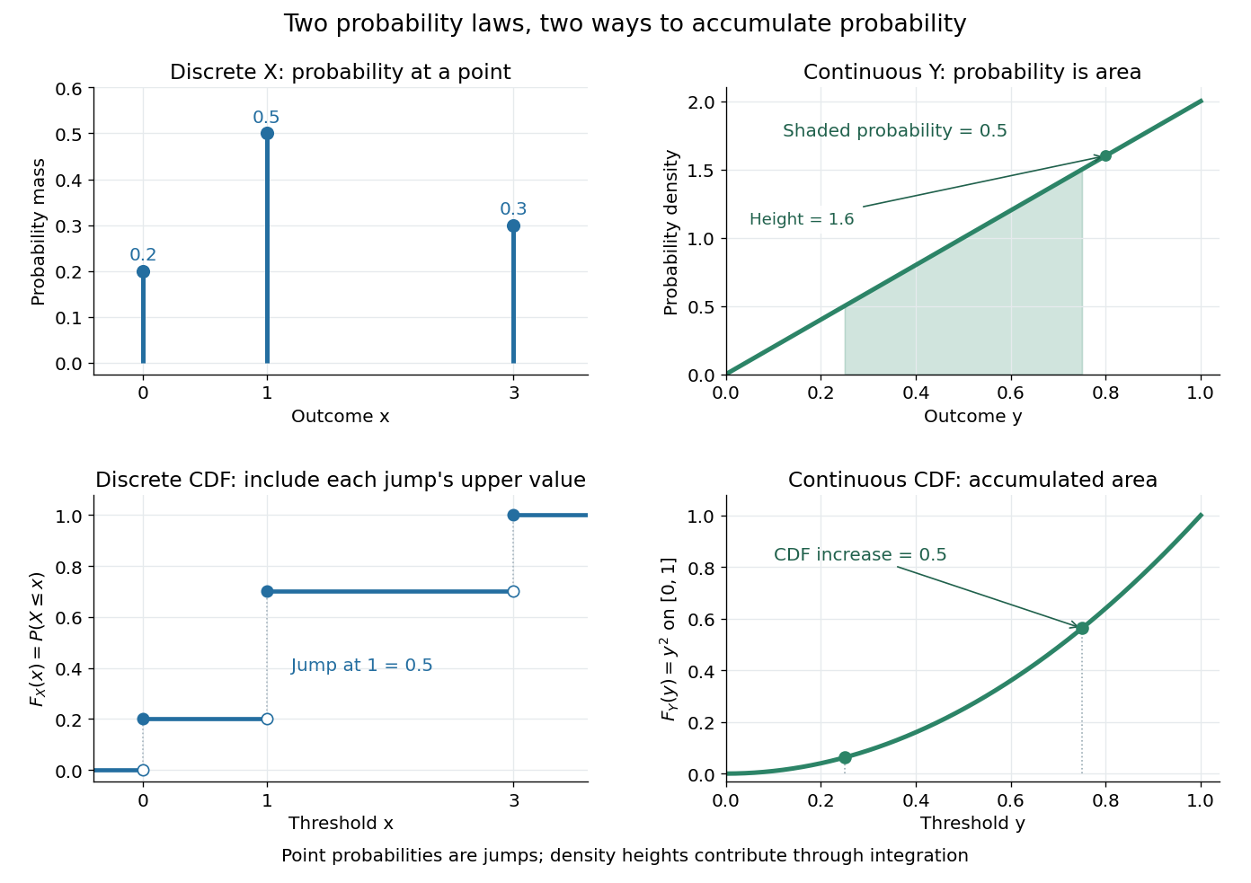
The cumulative distribution function answers all threshold questions for a real random variable, regardless of whether there are jumps or a probability density function. A quantile function reverses the direction of the question: given a cumulative probability level, find a threshold. This connects descriptive summaries to inverse transform sampling, which constructs a chosen probability distribution from a uniform distribution.

Total variation distance asks how much two probability distributions can disagree about the same event. For probability measures $P,Q$ on one measurable space $(S,\mathcal{F})$, its definition isThe supremum ranges over all measurable sets, so $d_{\mathrm{TV}}(P,Q)\le \epsilon$ guarantees that every yes-or-no prediction has probability error at most $\epsilon$. This metric takes values between zero and one; it is zero exactly when the two probability measures agree. This makes it useful for comparing a sampling algorithm's output with its target probability distribution, and for defining the mixing time of a Markov chain.

On a finite set, add the excess probability mass wherever $P$ exceeds $Q$. That excess is also half the sum of all absolute differences:The last expression reveals the common probability mass that the two probability distributions can share.^[ref] The coupling characterization of total variation distance turns this overlap into an actual joint construction; minimum sum of errors in a simple hypothesis test gives it a statistical interpretation. One quantity connects probability bookkeeping, comparison of sampling methods, and the limits of a statistical test.