This paper was printed as Algebra, Analysis and Differential Equations I and was shared by mathematics and mathematics and statistics. Source: released examination archive, member
FOI-20210708-1 - Data/4301 (1).pdf, pages 1–4. The examination took place on 18 June 2012. No mark allocations are printed. The solutions cover all nine questions.The dual space consists of the linear functionals on the original vector space, with addition and scalar multiplication defined pointwise:The dual map acts by function composition with :For , its value is . The composite is a linear functional because both and are linear maps. Moreover , so the dual map is itself a linear map. Its direction is reversed because a measurement on the output of becomes a measurement on its input.
The annihilator of a vector subspace consists of the linear functionals that vanish on every element of that vector subspace:For the dimension identity, choose a basis of and use basis extension to obtain for . A linear functional is determined by its values on these basis vectors. Belonging to the annihilator of a vector subspace sets its first values to zero and leaves its last values arbitrary. Equivalently the last elements of the dual basis form a basis of .
For a linear functional , the definition of the dual map givesThus the kernel of a linear map is precisely the annihilator of a vector subspaceWrite , and . The rank-nullity theorem, the dimension formula for an annihilator of a vector subspace, and giveApplying the same dimension formula in givesFinally, if and , then . Therefore . These are finite-dimensional vector subspaces of equal dimension, so inclusion is equality:This is the dual image and kernel annihilator identity.
A diagonalizable matrix over the field admits an invertible matrix with entries in such thatEquivalently, the vector space has a basis of eigenvectors of . Indeed, says that each column of is an eigenvector with the corresponding diagonal entry as its eigenvalue. Requiring the basis and eigenvalues to lie in makes the choice of field essential.
Expansion down the last column gives the characteristic polynomialThe quadratic polynomial has roots , which are not rational numbers. For example, the rational root theorem restricts any rational root of this monic integer polynomial to or , and neither works. If had a diagonalization over , its characteristic polynomial would be a product of linear factors with rational numbers as their roots. It is not, so is not diagonalizable over .
Over the complex numbers, the eigenvaluesare distinct. Thus distinct eigenvalues imply diagonalizability, and is diagonalizable over , in fact already over .
An explicit eigenbasis isFor either quadratic root , the identity verifies . Taking these three columns as gives . Their distinct eigenvalues ensure linear independence.
In the finite field , the characteristic polynomial becomesbecause modulo . Splitting into linear factors does not by itself guarantee diagonalizability: the repeated eigenvalue needs enough eigenvectors.
Solving givesso and . Hencehas dimension one, although has algebraic multiplicity two. The geometric multiplicity is too small, and is not diagonalizable over . This illustrates diagonalizability depends on the field: characteristic zero gave three distinct eigenvalues, while reduction modulo merges two of them.
A prime ideal is a proper ideal such that implies or . A maximal ideal is a proper ideal such that there is no ideal strictly between and .
Every ideal of the integers has the form for a unique nonnegative integer . Its prime ideals and maximal ideals are respectivelyThe zero ideal is a prime ideal because the integers form an integral domain. For a prime number , divisibility of by forces divisibility of one factor, so is a prime ideal. Also any ideal containing has , so it equals or ; thus is a maximal ideal.
If is composite, write with . Then while neither factor belongs to , so is not a prime ideal. A prime number gives , so is not a maximal ideal either. The zero ideal is not maximal since , and is not proper.
If the quotient ring is an integral domain, then , because an integral domain has . For ,There are no nonzero zero divisors in an integral domain, so or . Thus or , proving is a prime ideal.
If is a field, again is proper. Let be an ideal properly containing , and choose . The nonzero element has a multiplicative inverse , so . Since , subtraction gives , hence . Therefore is a maximal ideal. These arguments establish the relevant prime ideal quotient criterion and maximal ideal quotient criterion.
Set to define a surjective ring homomorphismIts kernel of a ring homomorphism is exactly : the constant coefficient in must vanish, so every remaining monomial is divisible by . The first isomorphism theorem for rings therefore givesThe polynomial ring is an integral domain, because the product of two nonzero polynomials has nonzero leading coefficient. It is not a field: has no polynomial multiplicative inverse, since a nonzero product has positive degree of a polynomial. Consequently is prime and is not maximal. Concretely, is a strict chain of ideals.
A subset is an open set if every admits a radius such that the open ballis contained in . A subset is a closed set if its complement is an open set. Equivalently, contains the limit of every convergent sequence of its points.
The distance to a set is nonnegative and finite here: any fixed gives . For every , the triangle inequality givesTaking the infimum over yields . Interchanging and provesThus is a Lipschitz function with Lipschitz constant one, so it is continuous. In the epsilon-delta definition of continuity, choose .
Conversely, if , the definition of the infimum allows a choice with . The sequence is therefore a convergent sequence with limit . Since is a closed set, its limit belongs to . HenceClosedness matters: without it, zero distance to a set characterizes its closure, which can contain additional points.
Put . This is a closed set. First assume is nonempty. The Heine-Borel theorem makes the nonempty bounded closed set a compact set. By the preceding parts, is a continuous function and is strictly positive at every , because .
The extreme value theorem gives attaining its minimum. ThereforeThe equality with the distance between two sets follows by taking the two infima successively. Crucially, compactness supplies a point attaining the minimum; positivity at each point alone would not make an arbitrary infimum positive. This is the principle that a compact subset of an open set has positive distance from its complement.
If , its complement is empty. With the usual extended-real convention , the stated inequality holds in that case too.
A holomorphic function on the open set is complex differentiable at every point of : the limitexists independently of the direction of approach. Write . The Cauchy-Riemann equations areTo prove necessity, approach first with real , obtaining . Approach instead with for real , obtainingEquality of real and imaginary parts yields the displayed Cauchy-Riemann equations.
A sufficient condition is that and have continuous first partial derivatives throughout and satisfy the Cauchy-Riemann equations there. Indeed, real differentiability gives, for ,The Cauchy-Riemann equations imply , so this is . Dividing by proves complex differentiability and at every point. Merely having first partial derivatives and the equations at a point, without a suitable differentiability hypothesis, would not justify this argument.
For the continuously differentiable function , the specified Wirtinger derivative isA complex number vanishes exactly when both real and imaginary parts vanish. ConsequentlyThus the two real Cauchy-Riemann equations are one complex equation expressed by the Wirtinger derivative.
The continuously differentiable function is a particular solution, sinceIf is any solution, set . Then is continuously differentiable and its Wirtinger derivative vanishes. By the preceding part and the sufficient Cauchy-Riemann equations criterion, is a holomorphic function on all of , hence an entire function.
Conversely, every entire function has vanishing Wirtinger derivative, so addition of preserves the prescribed derivative. Therefore all solutions areThis is an inhomogeneous Wirtinger equation with holomorphic forcing: a particular solution plus an arbitrary element of the homogeneous solution space.
A conformal map preserves oriented angles between intersecting smooth curves at each point, with a nonzero local scale factor. A sufficient criterion is that be a holomorphic function on the domain and that everywhere there. Its first-order action then multiplies every tangent direction by the same nonzero complex number, combining a rotation and a dilation. A conformal bijection additionally requires injectivity and surjectivity onto the target.
For in the given half-strip,Thus and . Conversely every such has a unique argument in and unique radius in , giving , . HenceThe complex exponential is injective on , and its derivative never vanishes.
On , use the Joukowski map with a sign change,Sinceit maps into the upper half-plane. To prove injectivity, givesBoth moduli are below one, so and .
For surjectivity, take any in the upper half-plane and solve . The two roots have product one. Neither can lie on the unit circle, since there is real. Exactly one root therefore has modulus below one. For this root, the displayed imaginary-part identity forces , so it belongs to . Finally has no zero in . This proves the Joukowski map from the upper half-disc to the upper half-plane is a conformal bijection.
Composing gives the required conformal mapIts derivative is nonzero on , since the zeros of the complex sine are the real integer multiples of .
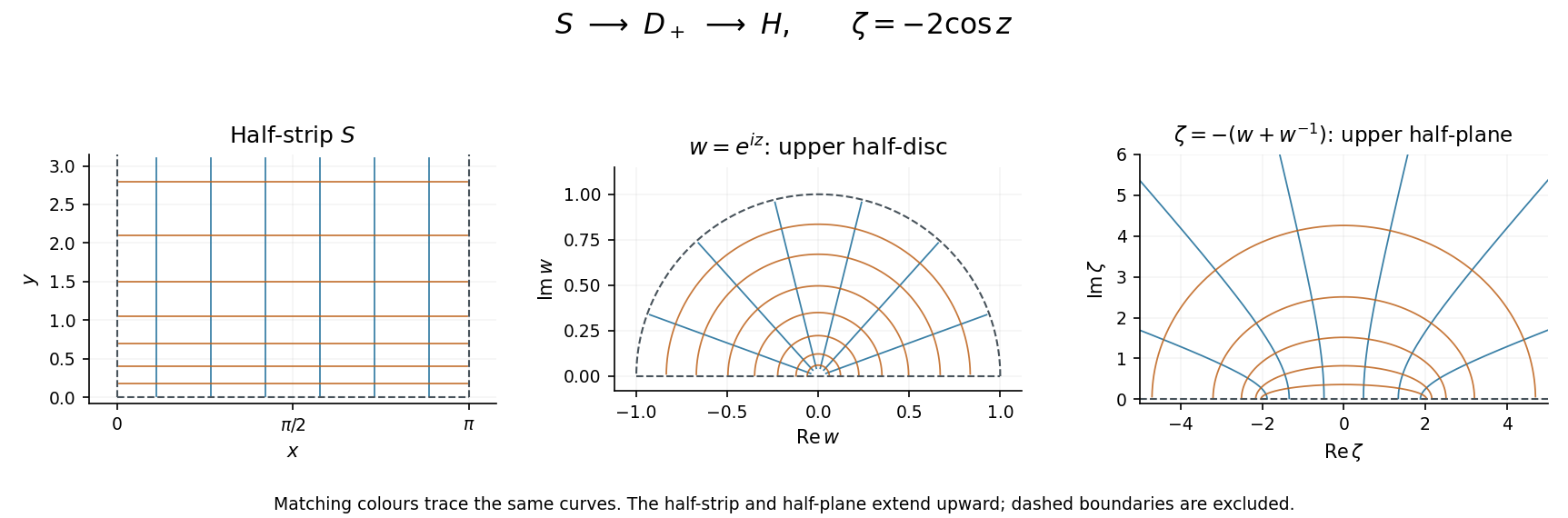
The half-strip maps to the upper half-disc by the complex exponential and then to the upper half-plane by a Joukowski map. Matching colours follow curves through both maps.
Details. 
Near , separation of variables gives , so . The initial condition selectsDirect substitution verifies both the ordinary differential equation and the initial condition. The endpoint is excluded because the coefficient and this solution are singular there; the displayed interval is the maximal connected real interval containing the initial point.
For and any two admissible values ,This is a Lipschitz condition in the dependent variable, uniform in , with Lipschitz constant . Also on the prescribed rectangle, so the usual local hypotheses of the Picard-Lindelöf theorem hold.
Integrating from the initial point gives the integral equationConversely, differentiating this equation using the fundamental theorem of calculus recovers the initial value problem. Start Picard iteration with the constant initial approximation and setThe first three approximations areTo prove the general expression by mathematical induction, put . The initial approximation gives the formula for . If it holds for , then the substitution rulegivesThus the formula follows at every stage.
For every fixed real , these are partial sums of the exponential series evaluated at the finite real number . ThereforeThis range is larger than : the expansion is in powers of , not a Taylor series in . For example it converges at . It also converges uniformly on every compact interval contained in , because is bounded there and the exponential series supplies a uniform summable bound. At the approximations are undefined, while for the real integral from zero crosses the singularity. This is Picard iteration for a simple-pole linear differential equation.
For a second-order linear partial differential equation with principal part , the discriminant is . Here , , , soThe equation is therefore a hyperbolic partial differential equation throughout its domain. The lower-order term does not affect this classification.
The characteristic curves satisfyIntegrating gives the two families . Choose coordinates constant along these families:Their Jacobian determinant is , so they define an invertible change of variables on , with image . Write . The chain rule givesBoth the pure second partial derivatives and the first partial derivatives cancel in the original equation, leavingThis is the full canonical form of a second-order partial differential equation, including the effect of the lower-order term. Integrating shows is a function of alone, hencewith arbitrary twice differentiable functions . The representation is global on : for each fixed , the allowed form an interval, so is independent of throughout that interval; after subtracting its antiderivative, the same reasoning in the other coordinate leaves only . These are quadratic characteristic coordinates for a variable-speed wave equation.
For the data on , set , so the other argument is . The two initial conditions becomeDifferentiating the first equation with respect to also gives . Solving these two linear equations yields . Since ranges over all real numbers,ConsequentlyIndeed , , , so the equation and both initial conditions hold directly.
For the Laplace transform of a derivative, first apply integration by parts on a finite interval:Under the usual transform hypotheses, including sufficient regularity for integration by parts, existence of the derivative's Laplace transform, and , passing to the limit givesThese conditions hold, for example, for a continuously differentiable with and of exponential order, in a sufficiently far right half-plane. Existence of alone does not establish all of these derivative-transform hypotheses; the finite-interval identity displays exactly which boundary term must disappear. The polynomial solution in the last part satisfies them for every .
For , the complex exponential tends to zero, since its modulus is . Therefore direct integration givesThe condition on the real part also gives absolute convergence of this improper integral.
Write . For , exponential decay dominates every fixed power of , so the improper integral converges absolutely and . For , integration by parts givesThe preceding part gives the base case . Repeated application, or mathematical induction, yields
Taking the Laplace transform, using linearity and the preceding three formulas, givesSince , division by gives for in the domain of convergence. There is no genuine singularity at : continuity of the Laplace transform there supplies the same value. One can also first work with , where division is harmless.
The formula in part (iii) identifies as the Laplace transform of . By uniqueness of the Laplace transform,As a direct check, and . Any two solutions of this initial value problem differ by and have the same initial value, forcing . This also verifies uniqueness independently of transform inversion.
Articles by others on the same topic
There are currently no matching articles.