Past exam of the algebra, analysis and differential equations II course of the University of Oxford / 2008 (AC2, XMAT 4302, XMST 4302)

Source: Mathematics release, bundle Part A 2007 11-1.pdf, pages 65–70. The six-page paper is shared by Mathematics and Mathematics & Statistics Part A, dated 17 June 2008. Its three printed sections are Algebra, Analysis and Differential equations.

Bounded exact-paper checks found no matching advertisement of worked answers. All nine questions, their printed parts, and their unnumbered tasks are answered. Full source statements remain in the private archive transcription.

Proceed by induction on $n=\dim V$. The zero-dimensional case is immediate. Over $\mathbb{C}$, the fundamental theorem of algebra supplies a root $\lambda$ of the characteristic polynomial. Since $\det (T-\lambda I)=0$, there is a nonzero vector $v_1$ with $T{v}_1=\lambda v_1$. The line $W=\mathbb{C}{v}_1$ is invariant, so $T$ induces a linear map $\overline{T}$ on $V/W$. By induction, choose an upper triangular basis for that quotient and lift its vectors to $v_2,\dots ,v_n$. Then $T{v}_j\in \mathrm{span}(v_1,\dots ,v_j)$ for every $j$. Thus $v_1,\dots ,v_n$ is the required basis and $\boxed{T\text{ is triangularizable}}$.

The same conclusion holds over $F$ when the characteristic polynomial splits over $F$. Indeed an eigenvalue then lies in $F$, and the block matrix arising from the invariant line gives ${\chi }_T(X)=(X-\lambda ){\chi }_{\overline{T}}(X)$. The quotient characteristic polynomial therefore also splits, so the induction works over $F$ without requiring algebraic closure.

Write $N=T-I$. Cayley-Hamilton theorem gives $N^3=0$. Its minimal polynomial is therefore $X^k$ for exactly one $k\in \{1,2,3\}$, so the possibilities for that of $T$ areLet $d=\dim \ker N$, which is the dimension of the only eigenspace. If $d=3$, then $N=0$ and $T=I$.

If $d=2$, rank-nullity theorem gives $\dim \mathrm{im}N=1$. The restriction of the nilpotent map $N$ to this invariant line is zero, so $N^2=0$. Choose $v_3$ with $v_2=N{v}_3\ne 0$, and choose $v_1\in \ker N$ independent of $v_2$. Then $v_3\notin \ker N$, so these three vectors form a basis; its matrix for $T$ is the printed $J_1(1)\oplus J_2(1)$.

If $d=1$, then $\mathrm{im}N$ has dimension two, so $N^2$ cannot vanish: otherwise $\mathrm{im}N\subseteq \ker N$. Choose $v_3$ with $N^2{v}_3\ne 0$ and set $v_2=N{v}_3$, $v_1=N^2{v}_3$. Applying $N^2$ and then $N$ to a putative linear relation proves these three vectors independent. The matrix is the printed $J_3(1)$.

These cases exhaust the possible eigenspace dimensions. They are pairwise dissimilar because similarity preserves the eigenspace dimension, equivalently the three different minimal polynomials. Hence every matrix is similar to exactly one of the three displayed forms.

The functional $\ell (u)=⟨u,v⟩$ is linear and nonzero because $\ell (v)=⟨v,v⟩>0$. It therefore has rank one, and rank-nullity theorem givesNo Gram–Schmidt argument is needed. Every vector decomposes uniquely as $u=w+av$, where $w\perp v$ and $a=⟨u,v⟩/⟨v,v⟩$. Substitution gives $S_v(w+av)=w-av$. Thus the eigenspace for $-1$ is $\mathbb{R}v$, and that for $+1$ is $v^{\perp }$. The latter is an actual eigenvalue when $n\ge 2$; when $n=1$ its eigenspace is zero and only $-1$ occurs. In the plane the map is reflection in the line perpendicular to $v$.

For equal-length crystallographic root configurations in a plane, taking $u=v$ in the closure condition gives $S_v(v)=-v$, so every vector occurs with its negative. For fixed $v\in \Phi$, a vector $u\in \Phi$ has $⟨u,v⟩\in \{-1,-1/2,0,1/2,1\}$, because both vectors are unit vectors. Thus its angle relative to $v$ belongs to the finite list $0,\pm \pi /3,\pm \pi /2,\pm 2\pi /3,\pi$.

If all vectors are collinear, the set is exactly $\{v,-v\}$, giving two opposite points of the unit circle.

If an orthogonal vector $w$ occurs, closure supplies $\pm v,\pm w$. A unit vector making an angle of $\pi /3$ or $2\pi /3$ with $v$ would have inner product $\pm \sqrt{3}/2$ with $w$, contradicting integrality of twice that inner product. Thus these four points are the whole set: the vertices of a square.

In the remaining case a noncollinear pair makes an angle of $\pi /3$ or $2\pi /3$. Changing a sign, take their angles as $0,\pi /3$. Reflecting the second in the line perpendicular to the first supplies the angle $2\pi /3$, and negation supplies the other three hexagon vertices. No perpendicular vector can occur, by the preceding inner-product obstruction. The initial finite list now leaves only these six points. Conversely the opposite pair, square and regular hexagon each satisfy both reflection closure and the integrality condition. Hence

For the polynomial ring, use the Euclidean function $\delta (f)=\mathrm{deg}f$ on nonzero polynomials. If $a,b\in F[X]$ and $b\ne 0$, subtract the multiple of $b$ that cancels the leading term of $a$. The leading coefficient of $b$ is invertible in the field, and every subtraction strictly lowers the degree of the remainder. This process terminates with $a=qb+r$ and either $r=0$ or $\mathrm{deg}r<\mathrm{deg}b$. Thus $\boxed{F[X]\text{ is a Euclidean domain}}$.

For the Gauss lemma for polynomials, call an integer polynomial primitive when its coefficient gcd is one. If two primitive polynomials had a nonprimitive product, a prime $p$ would divide every product coefficient. Reducing modulo $p$ would give a zero product of two nonzero polynomials in the integral domain ${\mathbb{F}}_p[X]$, a contradiction. Therefore the product of primitive integer polynomials is primitive.

To transfer a rational factorization, write each nonzero rational factor as a rational scalar times a primitive integer polynomial by clearing denominators and removing the coefficient gcd. Thus $f=qAB$ with primitive $A,B\in \mathbb{Z}[X]$ and $q\in \mathbb{Q}$. Their product is primitive by the lemma. If $q=m/n$ in lowest terms, integrality of every coefficient of $f$ forces $n$ to divide every coefficient of $AB$, so $n=1$. Hence $q\in \mathbb{Z}$; absorbing $q$ into either factor produces the required integer factorization with the same positive factor degrees. In particular irreducibility of a primitive polynomial over $\mathbb{Z}$ and over $\mathbb{Q}$ is equivalent.

Finally, let $a/b$ in lowest terms, $b>0$, be a rational root of a monic degree-$d$ integer polynomial. Multiplying the equation by $b^d$ shows $b\mid a^d$. Coprimality forces $b=1$. Thus $\boxed{\text{every rational root of a monic integer polynomial is an integer}}$.

An integral domain is a commutative ring with identity $1\ne 0$ and no zero divisors: $ab=0$ implies $a=0$ or $b=0$. Equivalently nonzero elements admit cancellation in multiplication.

A Euclidean domain is an integral domain equipped with a function $\delta :R\setminus \{0\}\to \mathbb{N}$ such that for every $a\in R$ and nonzero $b\in R$ there are $q,r\in R$ with $a=qb+r$ and either $r=0$ or $\delta (r)<\delta (b)$. One may additionally require $\delta (a)\le \delta (ab)$ for nonzero $a,b$; degree on a polynomial ring also satisfies this convention.

Let $h=f^{-1}$, $w_0=f(z_0)$ and $z=h(w)$. Continuity of $h$ gives $z\to z_0$ as $w\to w_0$, and injectivity gives $z\ne z_0$ when $w\ne w_0$. ThereforeThe assumed nonvanishing derivative makes this limit well defined. It exists at every $w_0\in V$, so $h$ is holomorphic, with $\boxed{h^{\prime }(w)=1/f^{\prime }(h(w))}$.

Squaring maps the first quadrant bijectively onto the upper half-plane. For $\zeta$ in that half-plane, $|\zeta -i|<|\zeta +i|$, and the Cayley transform $(\zeta -i)/(\zeta +i)$ maps it bijectively onto the unit disc. Their composition isThe inverse is the unique first-quadrant square root of $i(1+w)/(1-w)$, and is holomorphic by the first argument. Hence $H(w)=g(F^{-1}(w))$ is holomorphic throughout the disc. Its Taylor series at zero converges for $|w|<1$, locally uniformly there. Substituting $w=F(z)$ gives the stated expansion, with $c_n=H^{(n)}(0)/n!$, convergent at every point of the quadrant and locally uniformly on it.

If a holomorphic bijection existed, its inverse would be an entire function taking values in the unit disc. Liouville theorem would make that inverse constant, contradicting bijectivity. Thus no holomorphic bijection exists.

A continuous bijection does exist, even a homeomorphism:Both maps preserve the argument and change the radius by the mutually inverse strictly increasing functions $r\mapsto r/(1-r)$ and $s\mapsto s/(1+s)$. The displayed formulas also prove continuity at zero and everywhere else.

An isolated singularity at $a$ means that the function is holomorphic throughout some punctured disc $0<|z-a|<r$. Its residue is the Laurent coefficient $c_{-1}$, equivalently $(2\pi i{)}^{-1}{\int }_{|z-a|=\rho }f(z)dz$. The singularity is removable if all negative Laurent coefficients vanish, a pole of order $k$ if only finitely many are nonzero and the lowest power is $-k$, and essential if infinitely many negative coefficients are nonzero.

For the final contour integral, expand $e^{tz}{e}^{t/z}$. On the circle these exponential series converge absolutely and uniformly for $t$ in every bounded set, so their product can be integrated term by term. Inonly $j-k-2=-1$ contributes. Set $k=m$, $j=m+1$. ThusThe resulting power series converges for every complex $t$ by the ratio test. The coefficients are independent of the positive radius $R$.

Both numerator and denominator have simple zeros at zero, and $1-e^{-z}=z+O(z^2)$. Their quotient tends to one and extends holomorphically with that value. Hence the singularity is removable, and $\boxed{{\mathrm{Res}}_{0}f=0}$ because its Laurent series has no negative powers.

Use $\sin z=z+O(z^3)$ andTheir product is $z^{-2}+(3/2)z^{-1}+O(1)$. Thus the singularity is a pole of order two, with $\boxed{{\mathrm{Res}}_{0}f=3/2}$.

The denominator vanishes at $z_k=1/(2\pi ik)$ for every nonzero integer $k$. These points approach zero, the denominator has a simple zero at each, and $\sin z_k\ne 0$ because a nonzero purely imaginary number is not a zero of sine. Hence there are poles arbitrarily close to zero. The origin is a nonisolated singularity, so it has no residue defined by a Laurent series on a punctured disc. In particular it must not be classified as an isolated essential singularity merely because $e^{1/z}$ has one.

The identity theorem for holomorphic functions says that a holomorphic function on a connected open set which has distinct zeros accumulating at a point of the set is identically zero. Equivalently, two holomorphic functions agreeing on such a set of points agree everywhere in that connected open set.

To prove it, expand at an accumulation point $a$. If the first nonzero Taylor coefficient had index $m$, the function would factor as $(z-a{)}^{m}h(z)$ with $h(a)\ne 0$. Continuity would make $h$ nonzero near $a$, so no other zeros could approach $a$, a contradiction. Thus all coefficients vanish and the function vanishes on a neighborhood of $a$. Let $E$ be the set of points having such a zero neighborhood. It is nonempty and open. If a point in the domain is a limit point of $E$, it is either already in $E$ or is an accumulation point of distinct zeros, and the same Taylor argument puts it in $E$. Thus $E$ is relatively closed as well. Connectedness forces $E$ to be the whole domain. Apply this result to the difference of two functions for the equivalent formulation.

The given distinct zeros converge to $i$, which lies inside the connected upper half-plane. The identity theorem for holomorphic functions forces the function to vanish identically. Thus $\boxed{\text{no}}$.

Here the zeros accumulate only at the boundary point zero. An explicit holomorphic, nonzero example on the upper half-plane isAt $z_n=i/(n+1)$ its argument is $\pi (n+1)$, so it vanishes. It is holomorphic because the only excluded point of its formula is zero; it is not identically zero, for instance at $z=2i$. Thus the answer is yes.

The domain has two connected components. The zeros force the function to vanish on the upper half-plane but impose nothing on the lower one. DefineThis function is locally constant and hence holomorphic on the stated open set, and is not identically zero on that whole set. Thus the answer is yes. Connectedness is exactly the missing hypothesis for a global identity conclusion.

Differentiate the Wronskian:It is therefore constant. Linear dependence plainly makes it zero. Conversely, if it is zero, the two initial-data vectors $(u(0),u^{\prime }(0))$ and $(v(0),v^{\prime }(0))$ are linearly dependent. Some constants $A,B$, not both zero, make $Au+Bv$ and its derivative zero at zero. Uniqueness for a linear second-order equation with continuous coefficients then makes $Au+Bv$ identically zero. Thus $\boxed{w=0⟺u,v\text{ are linearly dependent}}$.

For the prescribed integral put $K(x,s)=[u(x)v(s)-u(s)v(x)]/w$. Then $K(x,x)=0$, $K_x(x,x)=-1$, and $K_{xx}(x,s)=-q(x)K(x,s)$. Differentiation under the integral, using continuity of the coefficients and forcing, givesThis proves the required inhomogeneous equation, with the sign of the forcing as printed.

For the explicit forcing take $u=\cosh x$, $v=\sinh x$, so $w=1$ and $K(x,s)=-\sinh (x-s)$. Since $2/(e^s+e^{-s})=\mathrm{sech}s$, the integral isIndeed expand $\sinh (x-s)=\sinh x\cosh s-\cosh x\sinh s$ and integrate $1$ and $\tanh s$. Adding the entire homogeneous solution givesFinally multiply the other equation by $\sin x$ and integrate from zero to $\pi$. Integration by parts givesThus $\boxed{{\int }_0^{\pi }f(s)\sin sds=0}$ is necessary. It is also sufficient: the solution with $y(0)=0$ is $B\sin x-{\int }_0^x\sin (x-s)f(s)ds$, and the integral condition gives its value zero at $\pi$.

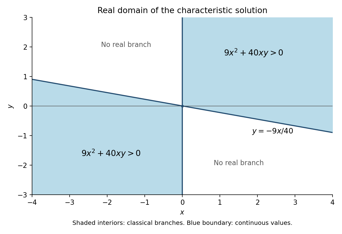
Use the characteristic parameter $t$ and writeDirect differentiation givesA characteristic beginning at $(s,0,0)$ therefore satisfies $5x+4y+3u=5s$ and $x^2+y^2+u^2=s^2$. Eliminating $s$ givesIts discriminant as a quadratic in $u$ is $100(9x^2+40xy)$. Requiring the root to be zero when $y=0$ selectsThe selected branch is differentiable in each of the two regions where the radical is strictly positive, and substitution into the differentiated quadratic identity verifies the partial differential equation there. On the initial line away from the origin the characteristic vector has nonzero $y$ component $-3s$, so these are the locally unique branches determined by that line.

The maximal real-valued continuation of these branches has the printed domainAt $x=0$ the continuous limiting value is $u(0,y)=3y/4$. The two bounding lines are $x=0$ and $y=-9x/40$, and the included sectors are the one above the sloping line on the right and the one below it on the left.

As in the fold boundary of a characteristic graph, the closed-domain statement concerns the formula's real values. A classical solution requires first derivatives on an open set. Along the nonzero boundary points $9x^2+40xy=0$, the radical's transverse derivative is singular, so the formula is generally not a classical solution there; its two classical domains are the interiors of the shaded sectors. The origin is characteristic for the initial data and does not supply a differentiable neighborhood solution. This qualification preserves the source's stated closed set while distinguishing it from the domain of a classical solution.

A critical point is an equilibrium: $\boxed{f(a,b)=g(a,b)=0}$. Put $X=x-a$, $Y=y-b$. The Jacobian matrix $J$ gives the first-order linearized equation $(\dot{X},\dot{Y}{)}^{\mathsf{T}}=J(X,Y{)}^{\mathsf{T}}$. The following eigenvalue tests classify that linearized system. For a continuously differentiable nonlinear system, the cases with nonzero real parts persist as the usual local node, saddle or spiral classifications. The purely imaginary case needs extra nonlinear information, as explained in (iv).

Both eigenvalues are real and negative: $\boxed{{\lambda }_1<0,{\lambda }_2<0}$, with distinctness as assumed. The two independent real eigendirections carry exponentially decaying factors $e^{{\lambda }_{j}t}$, giving a stable node.

Both eigenvalues are real and positive: $\boxed{{\lambda }_1>0,{\lambda }_2>0}$. The real eigendirections carry exponentially growing factors, giving an unstable node.

The eigenvalues are real and have opposite signs: $\boxed{{\lambda }_1{\lambda }_2<0}$. One eigendirection contracts and the other expands, giving a saddle.

For the linearized system a centre occurs when $\boxed{{\lambda }_{1,2}=\pm i\beta ,\beta \ne 0}$. Its real solutions are periodic ellipses after an invertible linear coordinate change.

As explained by a centre in the linearization need not be a nonlinear centre, for a nonlinear system these eigenvalues alone do not guarantee a centre. For example $\dot{X}=-Y-X(X^2+Y^2)$, $\dot{Y}=X-Y(X^2+Y^2)$ has eigenvalues $\pm i$ at zero but polar equations $\dot{r}=-r^3$, $\dot{\theta }=1$, so trajectories spiral inward. Removing the cubic terms gives a genuine centre with the same Jacobian. Thus there is no eigenvalue-only sufficient condition for a nonlinear centre in the stated generality.

The eigenvalues are a nonreal conjugate pair $\boxed{\alpha \pm i\beta ,\alpha <0,\beta \ne 0}$. The factor $e^{\alpha t}$ contracts while the imaginary part produces rotation, giving a stable spiral.

The eigenvalues are a nonreal conjugate pair $\boxed{\alpha \pm i\beta ,\alpha >0,\beta \ne 0}$. The exponential factor expands while the imaginary part produces rotation, giving an unstable spiral.

The equilibrium equations are $x(1+x-2y)=0$ and $(x-1)y=0$. If $x=0$, the second equation gives $y=0$. Otherwise either $y=0$, giving $x=-1$, or $x=1$, giving $y=1$. Thus there are exactly three equilibria. The Jacobian isAt $(0,0)$ it is $\mathrm{diag}(1,-1)$: a saddle. At $(-1,0)$ it is $\left(\begin{array}{cc}-1& 2\\ 0& -2\end{array}\right)$, with eigenvalues $-1,-2$: a stable node. At $(1,1)$ it is $\left(\begin{array}{cc}1& -2\\ 1& 0\end{array}\right)$, with characteristic polynomial ${\lambda }^2-\lambda +2$ and eigenvalues $(1\pm i\sqrt{7})/2$: an unstable spiral. All three are hyperbolic, so the nonlinear local classifications follow from linearization.

Suppose a nonconstant periodic orbit exists for the continuously differentiable planar vector field. Uniqueness implies that its image over a minimal period is a simple closed curve, enclosing a region $\Omega$ of positive area. Along the orbit, the differential form $fdy-gdx$ vanishes because $dx=fdt$ and $dy=gdt$. Green's theorem, with positive orientation, therefore givesa contradiction. This is the Bendixson-Dulac criterion in the whole plane; the fact that the enclosed region also lies in the domain is essential.

For the second-order equation set $y=\dot{x}$. The equivalent system is $\dot{x}=y$, $\dot{y}=-(1+x^2)y-\cos x$. Its divergence is $\boxed{-(1+x^2)<0}$ throughout the plane. Hence there are no nonconstant periodic solutions.

The nonconstant qualification is necessary: the equilibrium solutions $x(t)\equiv \pi /2+k\pi$, $k\in \mathbb{Z}$, do exist and are periodic in the literal sense of satisfying every positive period. The source's usual dynamical interpretation of “periodic solution” here is a nonconstant periodic orbit.