The characteristic equation of the homogeneous linear differential equation is , giving the homogeneous solution . For the first forcing, a particular solution of the form gives , soThe initial conditions impose and , whence , . Thus the first solution isFor the second forcing, is already a homogeneous solution, so the usual exponential trial must be multiplied by . Substitution of the particular solution gives , hence . Now , and the initial conditions give , . Therefore the resonant solution isThe additional factor reflects resonance in a differential equation.
This is a separable differential equation. On the solution with , integration from the initial condition givesThe right side lies in , so taking its sine stays on the required branch. The solution isNear the origin, , so and the tangent line is horizontal. At the other end, , whileThus the curve has a vertical limiting tangent line as , even though is excluded from the domain.
For the direction field, the slope is nonnegative everywhere in the square. The segments are horizontal on and on , become steeper as increases at fixed , and become flatter as increases at fixed . Near they are almost vertical unless is correspondingly close to one. The excluded corner has no single limiting slope: the ratio depends on the path of approach.
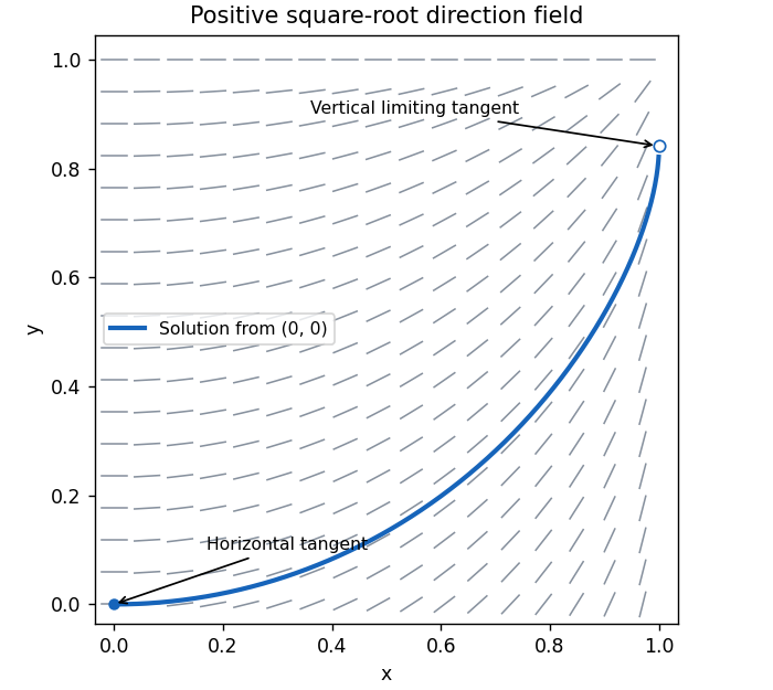
Positive slope field and the solution from the origin, with its horizontal and vertical limiting tangents
. Details. The indicator function equals one when the event occurs and zero otherwise. Its expected value is . By linearity of expectation, no independence assumption is needed to obtainSince , including , the variance isIn particular, correlations between the events cannot simply be discarded.
Write . If , then implies . Applying Chebyshev's inequality therefore givesEquivalently, the contribution of to is . A positive mean is necessary for the displayed ratio to be defined. If , nonnegativity instead gives almost surely, and the printed ratio would be .
After independent tosses, an even count arises in exactly two disjoint ways: an even count after tosses followed by a tail, or an odd count followed by a head. Independence of the last toss from the preceding ones therefore givesSubtracting the fixed point turns this into the linear recurrenceAs zero is even, , so the probability isFor this is for every ; for it is always one; for it alternates between one and zero according to the parity of .
An integrating factor for a differential one-form is a nonzero function for which is an exact differential, say . Then solutions lie on level sets . Locally, the compatibility condition is .
Here multiplication by , which is nonzero for , producesThe initial condition makes this first integral equal to . Taking the positive branch yields the solutionon the connected interval containing zero where the radicand is positive. This domain restriction matters because the original differential equation is singular at .
Completing the square gives . As , the differential equation consequently impliesAt , . Thus, moving a little to the left from , the curve rises above . Throughout every segment of the direction field points downwards as increases, by the inequality above. Tracing backwards therefore makes rise further, so it cannot return to . This graphical barrier argument proves and for every on the solution. The explicit first integral also shows this branch extends throughout : writing , the minimum of is , so for . Including the initial point, for all .
For the curve is on , where the strictly increasing function has the unique positive root at . The curve decreases through with slope and reaches only as a limiting endpoint. Its derivative isAs , and . As , the numerator tends to and the denominator to zero from above, so again . More precisely, at the endpoint. Both ends have the requested unbounded negative slope.
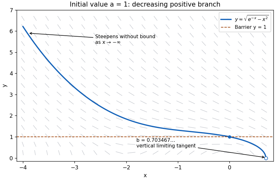
The positive solution for initial value one, with the horizontal barrier and the steep limiting endpoint
. Details. For the logistic differential equation, separate variables to obtain away from the constant solutions. Applying the positive initial condition givesThe formula also includes the constant solution . Below positive solutions increase; above they decrease. They approach as . Equivalently, linearizing gives and . Thus zero is unstable and is asymptotically stable.
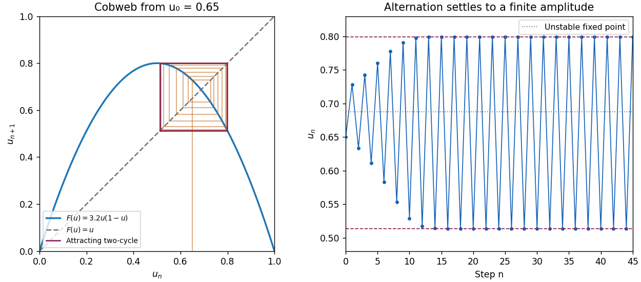
The forward Euler method gives . Set and ; multiplying the recurrence by this scaling factor gives the logistic mapIts fixed points are and . The fixed-point multipliers are and . Since , zero is always unstable. The positive fixed point is stable for and unstable for . For , a small displacement obeys : its sign alternates and its amplitude grows, giving an oscillatory instability whose period is .
This is an artifact of Euler discretization of logistic growth. Exact small perturbations decay by the positive factor per time step; a one-dimensional autonomous differential equation cannot have a nonconstant periodic orbit, since its solutions move monotonically between equilibrium points. The artificial instability occurs when , beyond the stable step range of this discretization.
For , remove the fixed point factors from to obtain . The resulting logistic map two-cycle isThese points map to each other. Their periodic-orbit multiplier is , so the two-cycle attracts nearby iterates. The cobweb shows a small initial departure from growing with alternating sign and then settling into the finite rectangle between and . The time trace shows the corresponding finite-amplitude oscillation.


Two functions are linearly dependent if constants , not both zero, satisfy identically. Differentiating also gives . Since the determinant of these two equations is the nonzero Wronskian , both constants must vanish. Hence the two solutions are linearly independent.
Differentiating the Wronskian and substituting the homogeneous linear differential equation givesIntegrating proves Abel's identity:For variation of parameters, impose on the proposed particular solution. Then , and substitution into the inhomogeneous differential equation leaves . Solving this two-by-two linear system givesArbitrary constants of integration merely add a homogeneous solution.
For the constant positive coefficient , take . Direct differentiation verifies that and solve the homogeneous linear differential equation; their Wronskian is . The requested integrands areTaking yieldsThus grows with power one, whereas is bounded. Their combination simplifies to ; the final sine term is itself a homogeneous solution. The secular term is the response to resonance in a differential equation.
Introduce . Along a solution,At , is a first integral. The identity shows its level sets are bounded: neither nor can escape to infinity on a fixed level. Consequently trajectories remain bounded as , including those starting far from the origin. This bound also prevents finite-time escape; no explicit solution is needed.
The equilibrium points are and . The Jacobian matrix at isAt the origin its eigenvalues are , with opposite signs, so the origin is a saddle point in all three cases. An eigenvector for lies on ; the stable direction has positive slope and the unstable direction negative slope. At the eigenvalues are .
When , these latter eigenvalues are . The nonlinear classification follows from the strict minima of at the two points: nearby level sets are closed curves without other equilibria, and the nonvanishing vector field makes them periodic orbits. Thus the two points are center equilibria. For , there are two separate closed ovals, one around each center equilibrium. The level consists of the saddle point and two homoclinic orbits forming a figure eight, explicitlyFor , a single outer closed orbit encloses all three equilibrium points. Motion is clockwise, as the vector points downwards wherever . The upper homoclinic orbit leaves the origin into and returns through ; the lower one has the reflected orientation.
When , the two nonzero equilibrium points have eigenvalues and are unstable foci. Nearby paths spiral outward clockwise. The first integral becomes a strictly increasing energy along every nonconstant trajectory: although can momentarily vanish when , it cannot vanish on an interval unless the solution is an equilibrium. Thus there are no periodic orbits or homoclinic orbits. The two stable separatrices of the saddle point, traced backwards, spiral towards the corresponding unstable foci. Its unstable separatrices move onto positive energy and escape outwards. All other nonequilibrium trajectories outside the stable manifold are unbounded forwards: a bounded forward limit set would have to lie in , whose only invariant points are the three equilibria; the two unstable foci cannot attract a nonconstant trajectory, and convergence to the saddle occurs only on its stable manifold. Escape is not finite-time blow-up, since bounds the energy on every finite interval.
When , the eigenvalues at the nonzero points are , so they are stable foci. The energy decreases, keeping all forward trajectories in compact sublevel sets. A bounded limit set must lie in the invariant part of , so trajectories converge to equilibria: generically to one of the two stable foci, exceptionally to the saddle along its stable manifold. The saddle's unstable separatrices spiral into the two stable foci; its stable manifold separates their attraction basins. Again, energy monotonicity excludes periodic orbits and homoclinic orbits. These three cases give the quartic double-well phase portrait with linear damping below.
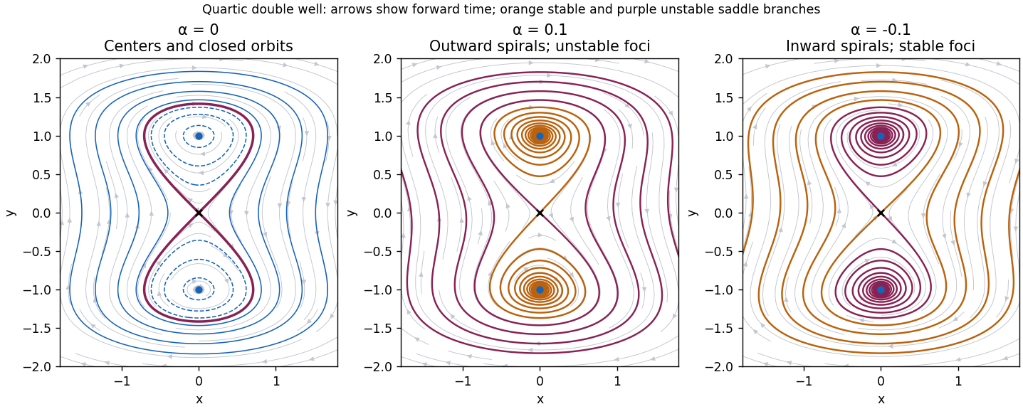
Conservative double-well closed orbits and the outward or inward spirals produced by positive or negative alpha
. Details. 
For , the conditional probability is . Since the events partition the sample space, their intersections with are disjoint and exhaust . The law of total probability therefore gives . Substituting this and into the definition proves Bayes' theorem:The denominator is positive by the given hypothesis on .
Every urn contains balls. Let be its number of blue balls; choosing an urn uniformly makes uniform on . Conditional on that urn, the probability of a blue first draw is , so the law of total probability givesDrawing twice without replacement requires . Given , the probability that both draws are blue is , and henceTaking the ratio defining conditional probability gives the second requested probabilityAlthough a blue first draw removes a blue ball from its urn, it also makes an urn rich in blue balls more likely. Averaging with this changed conditional distribution is essential.
Two independent events satisfy . If , this is equivalent to : learning that occurred does not change the probability of . The product definition also covers zero-probability events without dividing by zero.
The 36 ordered outcomes are equiprobable. For , let count outcomes with sum . Then and for . Their joint probability is if , and zero otherwise.
If the joint probability is zero, independence is impossible in these ranges because both marginal probabilities are positive. If it is , the independent events condition requires , or . This happens only for , and then all six values of allow the partner . Therefore within the possible sums and facesIf arbitrary integer labels outside these ranges are included, an impossible sum or face defines an empty event, which is trivially independent of every event.
Conditional on , the type indicators are independent random variables with the Bernoulli distribution of parameter . Thus has the binomial distribution and its probability generating function is . The general rule used here is that for a nonnegative integer-valued random variable , ; for a sum of independent such variables, their probability generating functions multiply, since the expected value of the product factors. The law of total expectation then averages the conditional result:This calculation uses the given independent labeling of objects, including conditional on their number.
A Poisson distribution with parameter has probability generating function . The preceding part gives , the probability generating function of a Poisson distribution with parameter . To prove independence, retain both counts:Consequently the joint probability generating function factors asComparing the coefficients of proves that the joint probabilities are the products of the marginal probabilities. Hence and are independent, with distributions and . This is Poisson thinning, including the degenerate counts when or .
With equal type probabilities, and have the same marginal probability generating function, namely . Their assumed independence, together with , givesSet for . The identity becomes and, after iterations,The finite expected value gives as . To justify this without any analyticity assumption at the endpoint, note that and is bounded above by ; dominated convergence gives the derivative . Substituting the expansion into the iterated identity yieldsThe left side is independent of , so it equals the limit. Thus on and uniqueness of the power-series coefficients proves . Only finite expected value was needed; the given finite variance is stronger. This proves the Poisson characterization by independent binomial splitting rather than assuming the original count distribution.
For independent random variables, the probability density function of a sum is the convolution of probability densities. Since each density is one on and zero elsewhere,This is the length of . Therefore the density isThe two triangular areas sum to one, as a probability density function must.
Conditioning on , independence of gives for and zero for . Using the preceding probability density function,
Three positive lengths form a nondegenerate triangle precisely when each is less than the sum of the other two. Necessity is the triangle inequality. For sufficiency, two circles centered at the ends of one side intersect off that side whenever the remaining lengths satisfy these strict inequalities, giving the third vertex.
Failure thus occurs when , , or . Two such inequalities cannot hold together for strictly positive lengths. Zero lengths and equality cases have probability zero because the variables have continuous probability density functions. By symmetry each failure event has the probability just calculated. Hence the probability of forming a triangle is
Another convolution of probability densities gives, for ,Only this part of the density is needed because the fourth length is at most one.
Four positive lengths can form a nondegenerate quadrilateral if and only if every length is less than the sum of the other three. Necessity follows by following the other three sides between the endpoints of the longest side and applying the triangle inequality. For sufficiency, select a diagonal length in the intersectionBoth intervals are nonempty, and their intersection is nonempty exactly when and . These are precisely the four strict length inequalities. Construct triangles with sides and on opposite sides of their common diagonal. Their union has the required simple, nondegenerate quadrilateral as boundary.
The failure events, in which one length is at least the sum of the others, are disjoint except on sets of probability zero. For the specified length , independence and the density above giveThere are four symmetric choices of the overly long side, so the probability isThis is the four-sided case of the polygon probability for independent uniform rods.
A branching process models reproduction through successive generations. In the Galton-Watson process used here, every individual independently produces a nonnegative integer number of offspring with a common offspring distribution; these reproduction counts are independent across individuals and generations. If is the generation size, thenwhere the have that distribution and the empty sum is zero. Thus zero is absorbing: once a generation is empty, every subsequent generation is empty.
Given , the next size is a sum of independent reproduction counts. Multiplication of their probability generating functions gives . Averaging this conditional expectation provesWith one initial individual, and , so is the -fold composition of with itself.
The binomial series givesThus and, for ,with the factors after omitted for . The signs follow from . As , the series has nonnegative terms and its sum increases to , so monotone convergence gives . These are therefore genuine probabilities on the nonnegative integers, proving that is a probability generating function. Its expected value is infinite, since ; finiteness of the mean is not required for this branching process.
Write . The composition formula gives , with . Consequently , and summing the geometric series yields the explicit generation generating functionThis is the fractional-power offspring generating function and its iterates.
Evaluation of the probability generating function at zero selects the constant coefficient, soTo identify this limit with ultimate extinction, let . The absorbing-zero property of the branching process gives . Ultimate extinction means that some finite generation is empty, namely . Continuity of probability on increasing events therefore givesThis set argument is essential: it uses absorption, rather than inferring extinction merely from a numerical limit of generation probabilities.
Articles by others on the same topic
There are currently no matching articles.