Use the normal linear modelHere is the response random vector, is the known design matrix, contains the unknown regression coefficients, and is the common error variance. Conditional on , the errors have normal distributions and are independent random variables. Require for identifiability of and invertibility of . Usually is needed to estimate the error variance from the regression residuals. An intercept, when included, is represented by a column of ones in .
Full column matrix rank makes a positive-definite matrix, and its matrix inverse is symmetric. Thus the hat matrix satisfiesAlso and the image of is contained in the column space of . These identities show that is the orthogonal projection matrix onto the column space of .
The ordinary least squares estimator is . Consequently the fitted values and regression residuals areAn affine transformation of a multivariate normal distribution is again multivariate normal, possibly with a singular covariance matrix. For a random vector with covariance matrix , its transformed covariance matrix is . Since , and , these results giveBoth multivariate normal distributions are supported on their respective projected subspaces. In particular, has variance and has variance ; the regression residuals need not be mutually independent.
Because both vectors are linear transformations of the same multivariate normal response, is jointly multivariate normal. Its cross-covariance matrix isZero cross-covariance implies independence for jointly multivariate normal vectors, including singular ones. Therefore the fitted values and the entire vector of regression residuals are independent. The fitted-residual orthogonality identity gives the zero covariance; the normal distribution assumption is what upgrades it to independence.
The simple linear regression assumes a straight conditional mean, , so that errors are centred at zero throughout the predictor range. The displayed regression residuals are predominantly positive at both ends and negative in the middle. This is a residual curvature diagnostic: the fitted straight line misses a curved conditional mean. The main concern is the shape of the mean function. The plot alone does not establish failure of the normal distribution assumption or a particular error variance model.
A natural next fit is quadratic regression, which remains a normal linear model in its unknown regression coefficients:The new design matrix has rows and must have matrix rank three; three distinct predictor values suffice. The curved regression residual pattern suggests trying a positive quadratic term, but its sign and adequacy should be checked after fitting. Inspect the new regression residuals to see whether the systematic curvature has disappeared.
Write . Apart from a constant, the log-likelihood isFor each group,Thus maximum likelihood estimation sets . The corner-point constraint identifies , givingThe baseline mean is the first group mean, rather than the grand mean, because of the chosen identifiability constraint.
Group means are independent random variables with normal distributionsThe resulting univariate sampling distributions areThe same variance calculation holds for every , since the difference involves two independent group means. Therefore the standard errors satisfyReplacing by a common estimated error standard deviation preserves this ratio. Although the individual group means are independent, the contrasts share the baseline mean and have covariance for distinct .
Index chocolate by , day by in the three observed categories, and replicate by . The additive two-factor normal linear model isHere is the board count, is the mean for the reference chocolate and reference day, and are chocolate and day fixed effects. With corner-point constraints, set and , where is the first level in the day factor. The printed coefficient-free output does not determine that factor ordering; the model is unchanged by a different reference category. There is no chocolate–day interaction term in this fit. The six free mean statistical parameters consist of one baseline, three chocolate contrasts and two day contrasts; the common error variance supplies a further statistical parameter.
Test for both nonreference days, against at least one nonzero day fixed effect, conditional on chocolate. There are two added regression coefficients and residual statistical degrees of freedom. The nested-model F-test statistic isUnder and the normal linear model assumptions, . Its 5% upper critical value is , so do not reject the absence of day effects; the p-value is approximately . Thus the missing row has two statistical degrees of freedom, mean square , and the F-test value above. These observations do not provide evidence that including day improves the chocolate-adjusted mean model. They do not prove that every possible day effect or chocolate–day interaction term is absent.
The analysis of variance provides evidence of a chocolate effect both with day included (, p-value ) and with day omitted (, p-value ). Because every chocolate–day cell has the same replication, balanced factorial orthogonality separates the two main effects; the chocolate row is meaningful despite being entered first.
The chocolate-only fitted group means are approximately boards for A, B, C, D respectively. Thus A has the largest fitted lecturing speed and C the smallest. Relative to A, the fitted differences are boards. The printed individual Student t-tests give strong evidence for the A–C contrast (p-value ); B and D versus A have p-values and , respectively. Those latter contrasts are not significant at 5%, and the output does not test all other pairwise comparisons. Simultaneous claims would require accounting for multiple hypothesis testing.
There is little evidence of a day effect after adjusting for chocolate. A chocolate-only normal linear model is therefore a reasonable simpler summary, with residual standard deviation about boards and explained variation . This is an association under the additive statistical model; a causal claim would additionally require an appropriate assignment of chocolate and checks of the regression residuals and possible interaction terms.
An exponential dispersion family has density or mass function, relative to a fixed measure,Here is the natural parameter, is the cumulant function, and is the dispersion parameter. Assume the natural parameter lies in the interior of its domain and derivatives can pass through the normalizing integral. Differentiating normalization once and twice givesThe variance function is , where the mean-to-natural-parameter inverse exists. The dispersion parameter may be fixed, as in a Poisson distribution, rather than estimated.
For and , the Poisson distribution has massMatch this to the exponential dispersion family withThen and . The canonical link function expresses the natural parameter in terms of the mean, so the Poisson canonical link is . Its conditional variance equals its conditional mean.
The coefficient labelled
yr2 identifies year as a factor. With in the first year and in the second, the Poisson regression assumes independent daily counts conditional on year,The unknown mean statistical parameters are the first-year log daily rate and the second-year log rate ratio ; the dispersion parameter is fixed at one. Approximate 95% Wald confidence intervals areExponentiating yields the first-year fitted daily mean , with confidence interval , andThe second-year fitted daily mean is . Thus this Poisson regression estimates a 9.35% fall, with an approximate interval for the percentage fall from 3.66% to 14.70%. These confidence intervals rely on the Poisson distribution and independence assumptions.The Quasi-Poisson regression retains the same conditional mean but permitsThis is a mean–variance function specification through quasi-likelihood; it does not assign a full probability distribution to each count. For independent observations, the quasi-score equation is proportional to , so the mean statistical parameter estimates equal those from Poisson regression. The output estimates through the Pearson dispersion estimator, and inflates the standard errors by approximately .
The large residual deviance relative to 728 residual statistical degrees of freedom also signals substantial overdispersion. Daily weather, traffic and other omitted conditions may produce greater count variation than a homogeneous Poisson distribution allows. The Quasi-Poisson regression accounts for that extra marginal variance. It still requires a correct conditional mean and an appropriate independence assumption; a common dispersion parameter alone does not repair serial correlation.
Under the more plausible Quasi-Poisson regression, the year Wald statistic is , with reported p-value . An approximate 95% confidence interval isThus the estimated fall is about 9.35%, but the data do not establish a reduction at the 5% level after allowing for overdispersion. The interval allows both a sizeable reduction and a small increase. The before–after comparison also lacks a contemporaneous randomized control, so causal inference about the campaign would require addressing other changes between years. The small Poisson regression p-value is not sufficient evidence of a campaign effect when its variance assumption is unsuitable.
Measurements from the same person share baseline strength and likely share an individual response to training. An ordinary linear model with independent errors treats all 600 readings as independent conditional on week; that fails to represent their within-person correlation. The regression residuals can remain associated even when the population mean is linear in time. A random intercept captures differences in baseline strength, and a random slope can additionally describe differences in progress.
For subject and , the random-intercept linear mixed model isAll subject random effects and measurement errors are mutually independent. The fixed effects describe the population mean baseline and weekly gain. Conditional on , a person's observations have independent normal distributions; after integrating out , their covariance is at distinct weeks and their common variance is . Therefore their correlation is .
This Gaussian linear mixed model permits correlated repeated readings while keeping different subjects independent. The fitted standard deviations are kg and kg, giving within-person correlation about . All persons still have the same latent weekly slope in this model.
Allow each subject to have a separate baseline and slope through a correlated random-intercept and random-slope model:The subject random effects are independent of all measurement errors, and subjects are independent. The within-person covariance between times is , with an additional when the same reading is used twice.
Prefer the model with a random slope. The maximum likelihood estimation refits improve twice the log-likelihood by while adding two covariance statistical parameters. Both the Akaike information criterion ( to ) and Bayesian information criterion ( to ) strongly favour it. The printed nominal likelihood-ratio test is overwhelming. The usual reference chi-squared distribution with two statistical degrees of freedom is not an exact regular calibration, since zero slope variance is a boundary and the intercept–slope correlation is then unidentified; a design-specific parametric bootstrap could calibrate it. This qualification does not undermine the substantial descriptive improvement shown by both information criteria.
The preferred fit estimates population mean baseline strength kg and weekly gain kg/week. The between-person baseline standard deviation is kg, and the between-person slope standard deviation is kg/week. Their estimated correlation is weakly positive, giving random-effect covariance about kg/week; its uncertainty is not supplied. The measurement-error standard deviation is kg. The printed instead describes the correlation between the estimated fixed effects, not between the subject random effects. These statistical parameter estimates come from restricted maximum likelihood; the model comparison uses the separate maximum likelihood estimation fits.
The population mean fitted trajectory is kg. HenceUsing the reported slope standard error, an approximate 95% confidence interval for the population mean gain is kg; a Student t confidence interval with 499 statistical degrees of freedom is almost identical.
Successful individuals can improve far more than the average. Their latent ten-week gains have fitted normal distributionA clear estimate for an upper-performing group uses a between-person slope quantile: the 95th percentile is kg, and the 97.5th percentile is about kg. The upper 5% of fitted underlying gains begin around 73 kg. These are person-to-person performance quantiles, not confidence intervals for the population mean. Identifying the best observed trainee would require that person's data or fitted subject random effects; the aggregate output cannot identify a literal maximum. If performance means the observed difference of endpoint readings, add the measurement-error variance to the latent gain variance.
Observed heterogeneity is variation in outcome propensities explained by measured covariates, such as age or sex. In logistic regression, subjects with different recorded predictor values may have different success probabilities, even before allowing for their previous outcomes. This is heterogeneity visible through observed predictors.
Unobserved heterogeneity is persistent variation between subjects arising from unmeasured characteristics. A subject-specific latent variable or random intercept can represent it. Subjects with high latent success propensities tend to succeed repeatedly, so their observed outcomes can have positive serial correlation even when outcomes are conditionally independent given that propensity. Apparent persistence therefore need not imply true state dependence.
True state dependence, also called true contagion, means that a previous outcome changes the distribution of a subsequent outcome after controlling both measured covariates and persistent unobserved heterogeneity. For example, an earlier successful week may make later success more likely through habit formation. A lagged-outcome coefficient in an inadequate statistical model can also reflect omitted subject differences, so positive observed persistence alone does not distinguish true state dependence from unobserved heterogeneity.
Let indicate a smoking-free week, the recorded sex indicator, age in years and assigned treatment. The screening history supplies ; earlier lag initializations are also zero. A history-dependent logistic regression for the first model isHere , is the observed past, and the five unknown regression coefficients have time-invariant values. Conditional on baseline covariates, this model has the first-order Markov property: only the immediately preceding outcome enters the current conditional probability. Distinct subjects have independent histories. There is no subject random effect or additional time trend in this fit.
Using the chain rule for probabilities, the individual conditional likelihood isThe lagged values in are the individual's actual preceding outcomes. This product is a sequential conditional likelihood, not an assertion of unconditional independence of the ten readings. The full conditional likelihood is ; no extra Bernoulli distribution factor is attached to the fixed screening history.
The second logistic regression adds while retaining the first lag and baseline covariates. The models are nested under . Their likelihood-ratio test statistic is the reduction in binomial deviance,Under the null and regular large-sample conditions for the correctly specified conditional likelihood, this has an approximate chi-squared distribution with one statistical degree of freedom. Since , reject at 5%; the approximate p-value is . Prefer the two-lag model to the one-lag model. Its additional lag captures statistically useful information in the history.
The cumulative-response logistic model uses instead of the two individual lag predictors. It and the two-lag history-dependent logistic regression are nonnested: the entire accumulated history generally cannot be represented using only the two recent outcomes. Their binomial deviance difference therefore has no ordinary nested chi-squared distribution calibration.
Use the Akaike information criterion, which up to the same saturated-model constant equals for these Bernoulli distribution conditional likelihoods. The two-lag fit has six coefficients, while the cumulative fit has five:Thus prefer the cumulative-history model, whose Akaike information criterion is lower by 35 despite its smaller number of statistical parameters. This is a model-selection comparison of conditional histories, not a nested likelihood-ratio test.
The preferred cumulative-response logistic model estimatesIts logit link describes conditional smoking-free probability given baseline predictors and prior successful weeks. Holding the other predictors fixed, males have times the female success odds; the reported p-value is , and the approximate 95% odds ratio confidence interval is . Age has estimated odds ratio per additional year, with p-value , giving little evidence for an age association in this fit.
The combined treatment has conditional success odds ratio versus the reference treatment, with approximate 95% confidence interval and p-value . The fitted conditional odds are about 39% higher for the combined treatment. The trial randomization supports treatment comparisons, but conditioning on accumulated post-treatment outcomes means this coefficient is not directly the marginal total treatment effect.
Each previous successful week multiplies current success odds by , with approximate 95% confidence interval and very small p-value . This is strong fitted persistence. It can reflect true state dependence, unobserved heterogeneity, or an omitted calendar-time trend; this fit alone cannot distinguish them. The baseline intercept implies success probability for a reference-treatment female aged zero with no previous success. That age is outside the study's useful interpretation range, so the intercept chiefly anchors the regression. The Bernoulli distribution dispersion parameter is fixed at one, and the residual binomial deviance is 1122 on 995 statistical degrees of freedom. With individual binary outcomes, comparing that binomial deviance mechanically to a chi-squared distribution is not a reliable general goodness-of-fit test.
Take the event to mean three smoking-free weeks in succession, . The initial cumulative count is zero. Along this path it equals in weeks one, two, three, respectively. In the cumulative-response logistic model, defineThe chain rule for probabilities then givesThe three conditional probabilities are approximately . If “stop during the first three weeks” instead means at least one smoking-free week by week three, its different event has probability : along the all-failure path the cumulative count stays zero. Stating the event resolves this wording ambiguity.
Let be the transition intensity from state to , and let be the transition intensity matrix, with . For a continuous-time multi-state model with the time-homogeneous Markov property, the transition probability matrix is , with entry . Condition on each recorded initial state. Panel visits contribute transition probabilities; an exact entry into the absorbing death state contributes a statistical probability densityThis mixed panel and exact-death likelihood sums over the living state just before death. It accounts for survival until the event; replacing its final factor by would count deaths throughout the interval.
Using the actual visit times recovered from the PDF, the three individual likelihood contributions areHere means with , not a transition probability. Subjects 8 and 9 supply no event-density factor after their last panel observation. Assume independent subjects and noninformative examination and censoring times; conditional on their observation schedule, its distribution supplies no additional statistical parameter-dependent factor. The patients' covariates can be incorporated by using their own in these same expressions.
For the progressive structure used in the subsequent output, put , , and . The progressive illness-death model permits no recovery, soWhen , the continuous limit is . Thus the likelihood contributions simplify toIntermediate unobserved disease transitions remain integrated into each panel transition probability.
The fitted progressive illness-death model has three allowed arrows: with estimated transition intensity , with , and with , all in years. State 3 is an absorbing state, and state 2 has no return arrow.
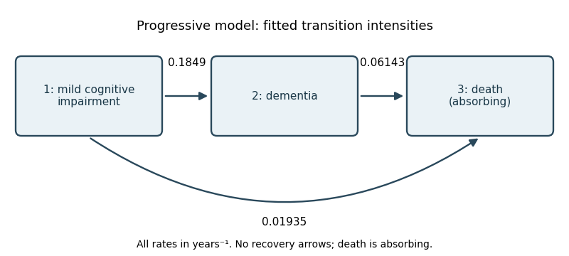
Progressive three-state model with estimated annual transition intensities
. Once in state 2, the holding time has an exponential distribution with rate , so the mean holding time from a transition intensity matrix isApply a confidence interval for an inverse rate to the printed rate interval : since inversion reverses order, the approximate 95% interval for the mean isThe time-homogeneous Markov property makes the future depend only on the current state; the exponential distribution also has the memoryless property. For a person currently in state 2,Equivalently, . Thus the fitted two-year death probability is approximately 11.6%.
Let contain sex, the education indicator, and age at diagnosis. Write for the sample means. The output's baseline transition intensities are evaluated at those means, so use the centred log-linear transition intensity modelThe full transition intensity matrix isThe fitted centred baselines are , and fitted slope vectors in sex–education–age order areThe two sex coefficients displayed as zero are fixed by the specified constraints; they are not estimated to be exactly zero. There are three free baseline transition intensities and seven free covariate slopes. The sample means are not printed, so uncentred intercepts at cannot be recovered numerically from this output.
Conditional on fixed covariates, subjects follow independent, correctly classified continuous-time multi-state models obeying the time-homogeneous Markov property, with . The progression is irreversible and death absorbing, with constant transition intensities during follow-up for each subject. In particular, the model uses fixed age at diagnosis rather than attained age. It assumes noninformative observation and censoring, and treats death times as exact through the mixed panel and exact-death likelihood. The Markov property rules out an additional effect of elapsed time in the current state after conditioning on it and the recorded predictors.
Under , the seven free covariate coefficients all equal zero. The likelihood-ratio test statistic isThe larger fit has ten free statistical parameters, compared with three in the constant-rate fit, so the reference chi-squared distribution has seven statistical degrees of freedom. Its 95th percentile is . Therefore reject at 5%; the p-value is approximately , and the covariate model is preferred. The two constrained sex coefficients add no free statistical parameters.
For the dementia-to-death arrow, the hazard ratio for higher versus lower education is , with approximate 95% confidence interval . Thus higher education is associated with a roughly 77.5% lower fitted death transition intensity, conditional on diagnosis age; the interval excludes one. This is an observational association and is not a direct multiplicative statement about death probability.
Each additional year of age at diagnosis multiplies the dementia-to-death transition intensity by , with confidence interval . The estimate suggests an increase, but the interval includes one, so this individual age coefficient is not significant at 5%. Sex has hazard ratio one for this transition by the model's imposed constraint. The output supplies no estimated sex effect or test of that constraint for this arrow. The nonzero sex coefficient for must not be mistaken for a sex effect on .
Articles by others on the same topic
There are currently no matching articles.