A weak white noise is a sequence with mean zero, a common finite variance , and for . A strong white noise is a sequence of independent and identically distributed random variables with mean zero and finite variance. Strong white noise is therefore weak white noise, but the converse need not hold. Neither definition, by itself, requires a Gaussian distribution.
For the spectral questions take the unique weakly stationary process solving the equation, as is customary for a stable autoregressive moving-average model. The equation alone also admits nonstationary solutions differing by , for which a spectral density of a stationary process need not exist. Let be the backshift operator. Since the autoregressive root is , the stationary solution is causal andUsing the convention , the spectral density of a stationary process isThe stationary mean is zero, since .
Here the innovation process consists of linear innovations, the linear one-step prediction errors: , where is the closed linear span of the past 's in . For Gaussian processes this is also the conditional expectation prediction error. For general non-Gaussian strong white noise these two notions can differ.
The given is not the linear innovation process. The moving-average factor has its zero at , inside the unit disk, and is noninvertible as a causal moving-average filter. The identityis the moving-average root reflection that places this zero outside the unit disk. Thus the causal invertible representation has innovation variance , rather than the given variance .
For an explicit verification, defineThe filter has constant squared modulus , so is weak white noise with variance . The new moving-average factor has root and is invertible, while its autoregressive factor is causal. Hence the past spans of and agree, and belongs to that past span. Orthogonality of to past therefore identifies it as the linear innovation process. The variance difference proves that it cannot be . If the original noise is Gaussian, the new linear innovations are independent Gaussian variables; without Gaussianity they need only be uncorrelated random variables.
The root-reflected, invertible autoregressive moving-average model isThis follows by multiplying the filter identity for by . Its moving-average root and autoregressive root are both outside the unit disk. Thus it is the representation in terms of the innovation process, rather than merely another noise representation with the same spectrum.
Expanding the stable autoregressive inverse gives the infinite moving-average representation in linear innovations:ThereforeFor comparison, the causal representation in the originally supplied noise isBoth converge in , since their coefficients are square summable. The second is causal, but its driving noise is not the linear innovation process.
Use the original-noise coefficients and for . The autocovariance function of a causal linear process is , since the original noise has variance . ThusFor ,By covariance symmetry,In particular, all nonzero-lag covariances are negative, despite the positive autoregressive coefficient.
The printed strong white noise assumption does not imply a normal distribution or even a finite fourth moment. Thus it does not, by itself, determine the covariance of a quadratic transform. We give the intended Gaussian calculation, and then the general finite-fourth-moment answer.
If is Gaussian, is a centered Gaussian process. Put and . Since and , the centered transform isThe supplied Hermite polynomial identity makes the cross terms vanish and givesEquivalently,The constant has no effect on covariance.
For a general iid noise with , put and , its fourth cumulant. Independence and expansion of third and fourth moments give, for ,whereSumming the geometric series explicitly givesThe covariance of quadratic transforms of a linear process follows from a fourth-moment expansion consisting of the three Isserlis theorem pairings, plus the fourth-cumulant contribution when all four noise indices coincide. The third-moment contribution similarly requires three coincident indices. This proves the general formula without assuming a normal distribution. For Gaussian white noise , recovering the simpler answer. If and the noise has infinite fourth moment, need not have finite variance, so an autocovariance function may not exist.
For a causal autoregressive model of order , the population partial autocorrelation function cuts off after lag , whereas the autocorrelation function generally decays. For an invertible moving-average model of order , the autocorrelation function cuts off after lag , whereas the partial correlation coefficients generally decay. For a mixed autoregressive moving-average model, both generally decay. Exponential decay may alternate in sign or show damped oscillations. Sample correlation coefficients only approximate these patterns, so isolated crossings of the significance bands are not exact order tests.
In PDF Figure 1, the autocorrelation function alternates sign, with a large negative lag-one correlation coefficient and geometrically decreasing magnitude. The partial autocorrelation function has essentially one substantial spike, negative at lag one and about ; later values mostly lie within the displayed bands. Thus a stationary AR(1) with a negative coefficient is the natural first model, with initially near . The trace fluctuates around an approximately constant mean and shows no evident deterministic trend.
Fit that model, compare nearby low-order alternatives using likelihood function and an Akaike information criterion or Bayesian information criterion, and inspect the residual autocorrelation function and residual variance. A few small later PACF spikes are expected in a plot with many lags. The roughly white noise bands are a guide, rather than simultaneous guarantees for every lag.
The sign alternation also suggests concentration of spectral power near the high-frequency end: the AR(1) denominator is smallest near when . From estimated and lag-one correlation coefficient one can estimate innovation variance as . The persistence parameter controls the decay rate and long-run variance of a stationary process. These plots do not establish a normal distribution, independence, or the absence of nonlinear dependence; correlation coefficients of squared residuals can provide a separate variance diagnostic.
With angular frequency , the periodogram isAt Fourier frequencies it is the squared modulus of the normalized discrete Fourier transform. If a nonzero mean is unknown, subtract the sample mean first.
For a zero-mean stationary process, expanding the square givesUnder absolute summability of the covariances this converges to the spectral density of a stationary process. Thus the periodogram is generally biased at finite , but asymptotically unbiased under this short-memory time series condition.
It is nevertheless not a pointwise estimator with statistical consistency unless it is smoothed. For Gaussian white noise, at a nonzero Fourier frequency other than the Nyquist frequency, the real and imaginary Fourier components are independent normal variables. Exactly,where . The variance does not decrease with . Under usual short-memory time series assumptions the same exponential limit is asymptotic for general processes. Averaging nearby frequencies or using a lag-window estimator reduces variance; a frequency bandwidth tending to zero while times that bandwidth tends to infinity can give statistical consistency. The raw plot remains useful for detecting strong periodic peaks, but increasing the record length alone does not remove its pointwise noise.
First, the absolute values in the printed limit are an error: the correct long-run variance of a stationary process is the signed sum of autocovariances. Directly,soEach coefficient tends to and has absolute value at most . Absolute summability and the dominated convergence theorem therefore giveThe sum of absolute values is an upper bound, not the general limit. For a concrete counterexample to the printed assertion, take with unit-variance iid noise. Then , , and other covariances vanish. The absolute sum is , but , so .
For correlated data the central limit theorem can still hold under suitable strong mixing of a stationary process and moment conditions, but the limiting variance is the long-run variance of a stationary process, rather than the one-observation variance. When it is positive,Positive serial dependence usually increases the standard error, while negative dependence can reduce it. The approximate effective sample size of a stationary sample is when that denominator is positive. A long-memory time series can require a different normalization or a different limit law. Absolute covariance summability alone does not prove a CLT: if with a common independent random scale taking values and with equal probabilities and iid with the standard normal distribution, the off-diagonal covariances are zero, yet has the nonnormal scale-mixture law . The example is not an ergodic stationary process. If the long-run variance of a stationary process is zero, the usual nondegenerate square-root- CLT is unavailable.
For the causal AR(1), andThe conditional distribution follows because the current innovation is independent of the past.
For a fixed known , condition on the observed and use the transitions . Their conditional maximum likelihood criterion is, up to constants,Differentiating in yieldsSince ,Thus it is an unbiased estimator, even conditionally on , andIt has statistical consistency with mean-square convergence, and the iid-noise strong law of large numbers also gives almost-sure statistical consistency. Its conditional distribution is exactly normal with the displayed mean and variance. If is also observed and all transitions are used, replace by .
The fixed- qualification is necessary for the exact finite-sample claims. If is jointly estimated, conditional likelihood function is linear regression with an intercept: writing and , the unconstrained estimators areThis ratio is not generally an unbiased estimator and does not have the preceding finite-sample variance. Under the usual stationary regression conditions it has statistical consistency; its asymptotic variance is . Indeed, it differs from by , an asymptotically negligible endpoint term. Profiling an unknown innovation variance does not change the fixed- estimate of .
The labels in PDF Figure 2 match as follows:Series has a wandering level and an overall upward drift. Its empirical autocorrelation function stays close to and declines very slowly, matching panel ; this is characteristic of a trend or a record from a unit-root autoregressive process. Such an empirical ACF is not a population stationary ACF if the underlying model is a random walk.
Series shows relatively smooth runs of adjacent observations on the same side of its level. Positive short-lag dependence emphasizes low frequencies, matching the decreasing spectrum .
Series is rougher, with much more rapid fluctuation. Negative short-lag dependence emphasizes high frequencies, matching the increasing spectrum . A negative-coefficient AR(1), for example, has this type of spectrum; the figure does not uniquely identify its exact order or parameters.
Series has conspicuous seasonality. Its autocorrelation function should alternate between positive peaks at full seasonal periods and negative troughs between them, matching . Here “characteristic function” is used descriptively for an ACF or spectrum, rather than for the probability-theoretic characteristic function of a random variable.
A nonstationary process has a statistical law that changes with the time origin. In the weak sense, this includes a time-dependent mean or variance, or a covariance that depends on the two times separately rather than only on their lag. A strictly stationary process requires invariance of every finite-dimensional distribution under a common time shift.
In the preceding plots, series suggests a stochastic trend or changing level, and series suggests a deterministic seasonal mean. These are the intended nonstationary examples. A plot alone cannot prove either conclusion: in particular, a stationary random-phase sinusoid can have a seasonal-looking trace and an oscillatory ACF. The interpretation of series as nonstationary concerns a seasonal mean tied to calendar time.
Three standard responses are to remove a fitted deterministic trend or seasonal mean; to use regular or seasonal differencing for an appropriate trend or seasonal component; and to stabilize a changing variance by a transformation or explicit seasonal scale model. For example, logarithms or a Box–Cox transformation can address level-dependent variance. The operation should match the source of nonstationarity; differencing a varying variance does not generally make it stationary.
Put and assume . ThenThus generally has a periodic mean, and generally has a periodic variance. The edge cases allowed by matter: is stationary when , because the mean is then constant, and is stationary for or . In the latter case multiplying iid centered Gaussian white noise by leaves its iid distribution unchanged. For every , but , so is nonstationary. For , is nonstationary because is not constant.
Use the seasonal difference operator . Since ,This is a stationary moving-average model of iid Gaussian white noise. Its covariance is at lag , at lags , and zero otherwise.
For the variance-modulated process the same operation givesIts variance is and its covariance at lag is . Therefore it remains nonstationary for , and the operation doubles the marginal variance at nonzero seasons. Seasonal differencing does not remove periodic variance: it removes a periodic mean, but the periodic variance generally remains. Practical alternatives are a periodic model or seasonal variance standardization; at seasons with the observations are deterministically zero, so division by is not possible there. For the already stationary special cases , filtering preserves stationarity.
A periodically correlated process with period has its mean and two-time covariance unchanged when both times are shifted by . For , the mean is zero andHence is a periodically correlated process. Its covariance period can be smaller than : when is even, , so is already a covariance period.
Use the usual normalization that is mean-zero unit-variance white noise orthogonal to the past, and extend periodically in . A nondegenerate causal periodic autoregressive model of order one requires . Write , with season indices understood modulo .
For , multiply the recursion by and use orthogonality of the current innovation to the past. The periodic Yule-Walker equations areAt lag zero, expansion of the squared recursion givesIn particular, , so an equivalent variance equation is . Negative lags are obtained from the given symmetry .
Replacing covariances by their sample versions givesTake the nonnegative scale and require a positive estimated predecessor variance. Using matched seasonal sample covariance matrices makes the quantity under the square root nonnegative by Cauchy-Schwarz inequality; with unmatched covariance estimates one can instead fit seasonal ordinary least squares and use the nonnegative residual variance. Statistical consistency of the covariance estimates gives statistical consistency of these plug-in estimators. If the driving noise variance were not normalized to , the equations would identify , not the two scales separately.
Draw independent uniformly on , and setThis is the Box-Muller transform. The endpoint has probability zero; an implementation should avoid evaluating its logarithm.
For , , so has density . It is independent of the angle, which has a uniform distribution on , and their joint density is . Transforming to Cartesian coordinates divides by the polar-coordinate Jacobian , yieldingThus the outputs are independent random variables with the standard normal distribution, proving the algorithm.
Let , and write for the standard normal distribution density. For importance sampling, choose the proposal density , namely the uniform distribution on the target interval. Its importance sampling weight isFor iid uniform draws ,is an unbiased estimator of the target mean, since its expectation integrates . If one chooses not to evaluate , the self-normalized importance sampling alternative has statistical consistency, but generally is not an unbiased estimator.
Alternatively, draw independent random variables with the standard normal distribution, let and , and useConditionally on , the retained draws are iid from the truncated normal distribution, so their average is an unbiased estimator with variance , where is its variance. If the ratio is undefined; one can continue drawing until a prescribed number of retained observations is obtained.
Here importance sampling uses every draw inside the interval, whereas only of the normal proposals are retained. The advantage can also be quantified. Integration using givesFor uniform importance sampling,For the retained-draw ratio with a fixed total proposal budget, its asymptotic variance coefficient is . Thus this importance choice has substantially smaller error for the same proposal count; it also avoids wasting about two thirds of the standard normal distribution draws. This comparison is specific to this well-matched importance sampling proposal; arbitrary proposal choices do not share this guarantee.
Use the spectral theorem for real symmetric matrices to write , with orthogonal and , . Set and generateThen . The characteristic function iswhich identifies the multivariate normal distribution . Equivalently, every linear combination is normal, with the required mean and variance. A Cholesky decomposition can be used for a positive-definite matrix. The spectral construction also works for singular , producing a degenerate Gaussian distribution on an affine subspace; in that case there need not be a density on all of .
Use as the variance parameter, with prior density relative to . Let and . Multiplying the prior by the likelihood function gives the unnormalized Bayesian posteriorThe printed request for an “improper posterior” should not be read as a claim that this posterior is always improper. Although the prior is improper, integrating over gives a marginal kernel , which is integrable exactly when and . Under these usual nondegenerate-data conditions it is a proper posterior. If those conditions fail, the displayed kernel is improper and there is no posterior probability distribution for a sampler to target.
Completing the square and using the inverse-gamma distribution give the full conditionalsThe inverse-gamma distribution convention is density proportional to . Equivalently the precision satisfiesusing shape and rate, as in the question.
A Gibbs sampler starts from and alternatesThis is the normal mean-variance posterior with a log-uniform variance prior. For a marginal check, : integrating out reduces the shape by . This marginal shape is different from the full-conditional shape .
Let be iid with density , set , and put and . The finite-second-moment assumption gives, for ,The sample variance consistently estimates . The central limit theorem and Slutsky theorem therefore give the asymptotic confidence intervalIts confidence probability is approximately , conventionally written ; the printed omits the factor . For , almost surely and the estimator has zero error. This interval concerns iid Monte Carlo estimators; correlated simulation output requires a long-run variance of a stationary process estimate instead of the iid sample variance.
The support condition for importance sampling is missing from the printed assertion. Assume , , and for -almost every . For a proposal , rejection has conditional probability . Its unconditional probability is , so the conditional density of a rejected draw isThus the rejected-draw weight is precisely , andConditionally on any positive rejection count among independent proposals, the rejected locations have this iid conditional density. Henceis an unbiased estimator conditionally on , and therefore also conditionally on the event . This is importance sampling from the rejected-proposal distribution.
The nonstrict assumption alone does not suffice: the rejected distribution may completely miss part of the target support. For example, let be uniform on , , , and . All rejected proposals lie in , where , so the displayed estimator is always , whereas . This remains a counterexample after conditioning on . A strict envelope, such as choosing larger than the essential supremum of , repairs the missing support condition. Near-equality can still give high-variance weights, even when it remains an unbiased estimator.
On , the exponential proposal is the proper density ; its integral is . The word “improper” in the question is therefore not applicable on its stated positive support.
The target-to-proposal ratio isIts maximum occurs at , so the smallest valid envelope constant isOne implementation draws and accepts it when , for independent random variables with the uniform distribution on . Accepted observations have the positive half-normal density by the usual rejection sampling calculation.
The printed identity needs an expectation on its right-hand side. For fixed , condition on and use independence of :The expression inside this expectation is generally random and cannot equal the unconditional probability by itself.
For each independent Monte Carlo method replicate, draw from its given distribution. If , draw independent -variables, form and set . For the empty sum is . If may equal zero, use when , since . The law of total expectation givesSince , the estimator has statistical consistency by the strong law of large numbers. It is the conditional Monte Carlo estimator obtained by Rao-Blackwellization of the direct indicator , and the law of total variance gives .
This version assumes that the cumulative distribution function can be evaluated. An easy sampler alone does not automatically supply an easy cumulative distribution function evaluation. If only sampling is available, use the direct indicator estimator, or replace each conditional cumulative distribution function by the average of several independent indicators ; the nested version remains an unbiased estimator. With such inner draws its variance per outer replicate is .
Let be a nonnegative target kernel and a proposal distribution. At state , propose , draw an independent uniform , and move to ifOtherwise keep . This is the Metropolis–Hastings algorithm. Start on the positive target support, with the usual zero-ratio conventions. The unknown normalizing constant cancels.
An unnormalized kernel is sufficient, provided . A genuinely improper target with infinite integral is not a probability density and cannot supply a stationary target probability distribution. The acceptance formula can still be written formally, but cannot be said to generate samples from that nonexistent probability law.
Because rejected proposals leave the state unchanged, the Markov kernel includes an atom:Detailed balance with a probability measure means the measure identityWhere both sides have ordinary densities, this reads . The measure formulation also includes the rejection atom. Integrating it shows that is invariant.
For the off-diagonal moves, the Metropolis–Hastings acceptance probability givesThis expression is unchanged by interchanging and . The rejected-move measure is supported on the diagonal and is also symmetric. Therefore the whole transition measure satisfieswhich proves detailed balance, including the atom that an off-diagonal density alone would omit. Consequently the Metropolis–Hastings algorithm kernel preserves the normalized target measure.
For coordinate , keep the other coordinates fixed and propose from the full conditional . This is a Metropolis–Hastings algorithm proposal on that coordinate fibre, with deterministic equality . Its acceptance ratio isThus the coordinate update has acceptance probability one and is exactly a single-coordinate Gibbs sampler update.
A systematic sweep through coordinates is the composition of these kernels. Its joint transition density isThe already updated coordinates are new values, and the not-yet-updated coordinates are old values. Each coordinate kernel preserves , so their composition also preserves it. Systematic Gibbs sampling need not be reversible: each individual coordinate kernel is reversible, but their ordered composition need not be reversible; invariance is the property needed here. A random-scan mixture of the coordinate kernels is reversible.
Use the ergodic theorem for a positive Harris recurrent Markov chain: for an invariant distribution and an integrable function , the time average converges almost surely to under the usual ergodicity conditions. This is the relevant theorem for correlated Metropolis–Hastings algorithm output, rather than the strong law of large numbers. Here is integrable. Indeed, puttingwe have , which bounds the unnormalized density by a constant times an integrable Gaussian density and also gives finite first moments.
For a proposal scale , initialize anywhere in . At each step draw independent random variables with the standard normal distribution and an independent uniform , propose , and accept whenOtherwise set . The normal proposal is symmetric, so its density cancels; the target normalizing constant also cancels. Include every state in the average, including repeated states after rejection. The ergodic theorem for a positive Harris recurrent Markov chain then givesA fixed discarded initial segment does not change this limit.
Small proposal variance gives high acceptance but tiny moves and strong serial dependence. Large variance gives more ambitious moves, but many proposals enter very low-density regions and are rejected, creating long runs at one state. An intermediate scale should be assessed by exploration and effective sample size of a Markov chain, not acceptance rate alone.
This density has two modes, at and their interchange. To see this, stationary points satisfy , implying either or . The unequal solutions have and are local minima of ; the equal solution is a saddle. Mode switching is therefore a material part of proposal-scale selection: a chain confined to one mode can have high acceptance and a misleading finite-run estimate.
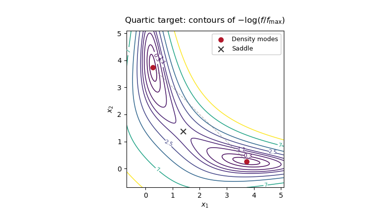
Two modes of the quartic target density, with the diagonal saddle between them, explaining slow mode switching in random-walk Metropolis-Hastings
. Details. 
Articles by others on the same topic
There are currently no matching articles.