For a differentiable vector field in Cartesian coordinates, the divergence and curl arewith summation over repeated indices. In components the curl is . The contraction of two Levi-Civita symbols and the product rule giveRecognizing the directional derivatives gives the curl of a cross product identity
The divergence is . Over the cube , each squared-coordinate term has integral , while the other two coordinate integrals have length one. ThusCompute the surface flux separately. On , the outward normal is and , giving flux . On , the normal is , so , again giving . The two faces similarly give each, and the two faces give each. All six face integrals therefore giveThe independently evaluated values agree, verifying the divergence theorem for this field and cube.
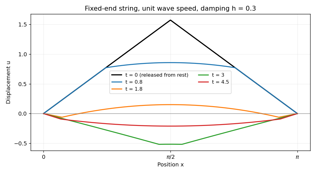
Use separation of variables . The fixed-end Dirichlet boundary conditions select , , and each mode satisfies . In the physical resistance range , all normal modes are underdamped, with . The modal factor normalized by , isConsequently the linearly damped string has solutionThe coefficients are those of the initial Fourier sine series. Differentiating each normalized modal factor at zero confirms that the string starts from rest. Suitable initial data give convergence in the string's energy space; the piecewise linear profile here need not give a twice differentiable solution along every characteristic from its corner.
For the specified tent profile, integrating its two linear pieces by parts givesFor example the first piece gives , and the second gives the opposite cosine term and the same sine term. HenceThe zero even coefficients also follow from reflection symmetry about the midpoint. This is the Fourier sine series of a symmetric tent. If were read without the physical assumption , the same modal solution extends by replacing imaginary-frequency sine and cosine by their hyperbolic counterparts, and taking when .
The homogeneous Cauchy-Euler equation has solutions and . Choose , which vanishes at zero, and , which vanishes at one. Their Wronskian is . For a Green function integrated against the unweighted measure , continuity at and the jump condition giveIt satisfies for . Therefore the candidate solution isThe leading coefficient vanishes at zero, so the endpoint condition needs care. If extends continuously to , this expression has limit as . Indeed and , while the remaining terms vanish. Thus the continuous zero-endpoint problem in this class requires . With that compatibility condition the formula gives both boundary values and is unique: a difference of two bounded solutions is , whose two endpoint conditions force both constants to vanish. For incompatible forcing such as , the bounded solution with is , which cannot also vanish at zero. Pointwise vanishing of for fixed does not justify interchanging the singular endpoint limit with its integral. This issue is treated in Green kernel and endpoint compatibility for a singular Euler equation.
For the supplied compatible forcing , the integrals are and . Their polynomial pieces cancel, givingDirect differentiation gives , and at zero. Its derivative diverges there, which is allowed because the boundary condition requires the value, not a finite derivative.
Choose the Fourier transform convention , with inverse . For absolutely integrable , Fubini's theorem permits the substitution in the convolution transform:This proves the convolution theorem in the chosen convention.
Take . Splitting its transform at zero gives . Thus the desired inverse is . For , split the convolution integral at and :The result is even, soDifferent normalization conventions alter the transform prefactors, which is why the convention was stated explicitly.
The spectral theorem for real symmetric matrices supplies an orthonormal basis of real eigenvectors. Put these in the columns of , so and . In the question's coordinate convention choose and . Since ,Reorder the eigenvalues with positive, negative and zero. For nonzero eigenvalues set , and retain the remaining coordinates as . This is an invertible real transformation , where is the diagonal rescaling; the combined matrix gives . It giveswith the zero coordinates absent. The general allowed range is . The printed restriction is not valid for every real symmetric matrix: a negative-definite or zero form has no positive square. The invariance of these counts is Sylvester's law of inertia.
For the specified form, a particularly simple change isSubtracting the first two squared coordinates verifies the identity directly, and proves invertibility. Thus , and there is one zero direction. The final rescaling need not remain orthogonal.
A square complex matrix is a unitary matrix when , so it preserves the Euclidean norm. If with , then , giving . For a Hermitian matrix and ,because the numerator equals its complex conjugate. Hence no eigenvalue of is zero, proving it is invertible.
For , the Hermitian conjugate is . The factors and their inverses commute, since they are rational functions of . Thus . Its action on the same eigenvectors isThese eigenvalues have modulus one. This is the Cayley transform of a Hermitian matrix in the convention that avoids the unitary eigenvalue one.
For the inverse direction, givesTaking the conjugate transpose of therefore yieldsThe last equality uses commutativity of the two factors. This proves that the inverse Cayley transform of a unitary matrix without eigenvalue one is Hermitian. Solving for gives . An orthonormal eigenbasis of therefore diagonalizes , with diagonal entries .
The result extends even when a unitary matrix has eigenvalue one: choose so that does not. There are only finitely many forbidden phases, since the matrix has finitely many eigenvalues. Diagonalizing also diagonalizes in the same basis. Thus every unitary matrix is unitarily diagonalizable.
Factor . The geometric series gives, for ,Thus the first three nonzero terms are . If “first three terms” means the coefficients through degree two, that Taylor polynomial is . The distinction matters because the quadratic coefficient vanishes. The nearest singularities are the two nontrivial cube roots of unity, so the radius of convergence is exactly one.
Put . The identity gives a Laurent series containing a constant and only even negative powers . There is no coefficient, soThe singularity is an essential singularity, not a pole: infinitely many negative Laurent coefficients are nonzero. The residue is still defined as the coefficient of .
For , fix one argument . Every value of the complex logarithm is , . By complex exponentiation, . Taking the real part of its exponent gives all possible moduli:Equivalently these are . If is real and nonzero the modulus is the single value ; otherwise the values form a geometric progression with ratio . Changing the initially chosen argument just reindexes the same set. The logarithmic definition excludes . This is the modulus of a complex self-power.
For a nonzero solution on a branch where the real power is differentiable, set . Multiplying the Bernoulli differential equation by gives the linear equationIt can be solved by an integrating factor. For the specified cubic equation take , , so satisfies . Its integrating factor is , giving and hence . Thus all nonzero real solutions areon connected intervals where the denominator is positive, with a fixed sign on each interval. Also solves the original equation and must be restored because the substitution excluded it. The choices give the constant solutions . Smoothness of the original right-hand side gives uniqueness, so a nonzero solution cannot cross through the zero solution at a finite regular point.
Write the analytic solution as . The constant term in the differential equation gives , and matching the coefficient of givesAll odd coefficients therefore vanish; and . The first three nonzero terms areIn full, , so , a Bessel function of the first kind. The ratio test proves convergence for every complex . The other independent solution has a logarithmic singularity at zero and does not satisfy the analyticity requirement.
Introduce a Lagrange multiplier for the constraint and vary with , where . The first variation isThe fundamental lemma of the calculus of variations gives the Sturm-Liouville equation . Multiplying by , integrating by parts and using the endpoint conditions gives . Therefore the normalization implies . Assume the coefficient and function regularity needed for these variations and integrations; the condition makes the constraint derivative nonzero at a normalized function.
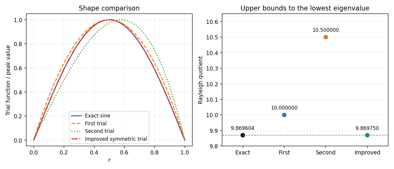
For the radial problem, set . A direct differentiation gives , soFinite supplies the first boundary value. The Rayleigh quotient is . For the two trials, and , the numerator-denominator pairs are and , respectively. HenceThe exact eigenvalues are , so . Both trials give upper bounds by the Rayleigh-Ritz variational principle, and the first estimate is more accurate, since it is smaller. Trial admissibility uses the Dirichlet energy form for ; the first trial's nonzero radial derivative at the origin does not invalidate this variational calculation.
To improve, add independent trial functions and minimize the quotient over their span. Here merely combining the two supplied trials gives no improvement: their two-dimensional stiffness and mass matrices areThe lowest Ritz value is still ten. Instead add the symmetric quartic . On the span of , the generalized eigenvalue problem hasIts determinant is , so the least root givesThis is strictly better than both original estimates. The symmetry obstruction in a polynomial Rayleigh-Ritz trial space explains why the cubic addition failed while the quartic helps. It is also the shifted-interval version of the polynomial Rayleigh-Ritz trial space for a one-dimensional box.
At a regular constrained extremum, the method of Lagrange multipliers makes stationary for a constant . For an endpoint-vanishing variation , integration by parts givesThe fundamental lemma of the calculus of variations therefore yieldsThis Euler-Lagrange equation must be supplemented by the two endpoint conditions and the prescribed integral constraint, which determine the constants and multiplier. Existence of the normal multiplier assumes that the first variation of is not identically zero. If that regularity fails, the general multiplier equation uses , with ; one cannot automatically set .
Write the speed as and takeThe two Euler-Lagrange equations areFor example and , yielding the first equation. Integrating once gives constants with and . The case would force both velocities to vanish, contrary to a regular curve. Squaring and adding therefore givesThus every regular stationary curve is a circle, whose center is set by the integration constants. A simple closed traversal of length has radius and positive enclosed area . The planar isoperimetric inequality proves that this stationary candidate is the global maximum; the necessary variational equations alone would not prove that inequality. The stationary curves of the planar isoperimetric problem give this argument independently of the chosen parametrization.
Use the standard regular self-adjoint assumptions on the Sturm-Liouville problem, including positive weight . The normalized eigenfunctions obey orthogonalityCompleteness means every function in the weighted space has expansion , with convergence in that space. Comparing the action of this kernel on test functions with the Dirac delta gives, in the distributional sense,If zero is not an eigenvalue, divide each term by . Since , application of recovers the displayed delta expansion, provingThe factor is required because the source equation uses an ordinary, unweighted delta. It distinguishes the normalized Sturm-Liouville spectral Green kernel from a kernel integrated against weighted source measure. If there is a zero eigenvalue, an inverse for arbitrary forcing does not exist; the unqualified division by that eigenvalue is invalid.
For with real and zero endpoints on , the weight is one, and . Substitution yieldsThe series is absolutely and uniformly convergent, although applying the differential operator is understood distributionally at its source point.
Set and multiply the Laplace equation by . Separation of variables givesWith , the angular equation is . Regularity at both poles selects the Legendre polynomials and . The radial Cauchy-Euler equation has solutions . Expanding the angular data in this complete orthogonal system therefore giveswith the usual convergence required of a harmonic expansion on the region considered. Angular Legendre functions singular at the poles are excluded.
For , the outer data have expansion , while the inner data are pure . Thus only degrees zero and two are needed. A radial interpolation matching each pair of boundary values givesThe first term is a linear combination of and takes values at the two radii. The second is a combination of and takes values zero and . These checks establish both boundary conditions; each term is harmonic. The maximum principle for harmonic functions gives uniqueness. This is an example of axisymmetric harmonic interpolation between concentric spheres.
Write . A radial function harmonic away from the source satisfies , hence . Decay at infinity forces . Integrating over a small sphere, the divergence theorem requires flux one:Therefore the fundamental solution in this sign convention isAdding point sources outside the domain changes only a harmonic function inside it. The method of images selects their positions and strengths to cancel boundary values. The sign reverses for the alternative convention .
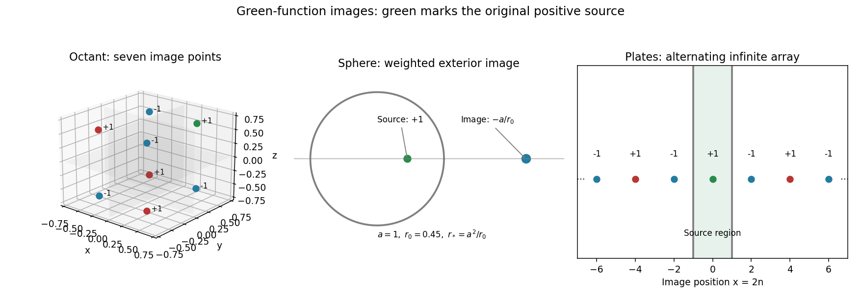
Let the source be with all three coordinates positive. Reflect it independently in the three coordinate planes: the eight points are , with . Assign strength . ThenThe all-positive point is the original source. On any boundary plane, two terms differing only in that plane's sign have equal distances and opposite strengths, so cancel. All seven additional points lie outside the positive octant, leaving exactly the required interior source. This is the octant Dirichlet Green function.
Let with . The Dirichlet Green function inside a sphere uses the exterior inverse point and strength . ThusFor , the distance identity makes the bracket zero. The image is outside the sphere, so it adds no interior singularity. This is the radial weight associated with the Kelvin transform.
The printed unit-strength restriction must be relaxed in this part: the required single image has strength , whose magnitude is generally not one. A reflected unit charge does not give the spherical boundary cancellation. For a centered source, the limiting formula isIts correcting term is constant and corresponds to the weighted image moving to infinity, rather than a finite unit point image.
Take the source at the origin and write . Repeated reflection in places the sources at with strengths , . There are countably infinitely many images; is the original source. A convergent prescription groups adjacent opposite charges:Each bracket is on compact sets away from the source, so the paired series converges absolutely. The individual unsigned point-charge terms would not be absolutely summable. On , reflection pairs the index with ; on , it pairs with . Their distances agree and signs oppose. Symmetric finite cutoffs leave only a vanishing far-tail contribution, proving both zero boundary values. All nonzero-index sources lie outside the slab. This is the centered-source version of the Dirichlet Green function between parallel planes, selected to decay at large transverse distance.
Cauchy's integral theorem states that a holomorphic function on a simply connected domain has zero contour integral around every closed piecewise smooth curve in that domain. One proof begins with the Cauchy theorem for a triangle. Subdivide a triangle into four equal triangles. Their oriented boundary integrals sum to the original integral because internal edges cancel, so choose a nested subtriangle carrying at least one quarter of the preceding integral's modulus. At stage , its perimeter and diameter are , and the nested triangles converge to a point . Complex differentiability gives , with . The affine terms have primitives and integrate to zero. Therefore , while . Letting proves . Triangulation cancels internal edges for polygonal contours; local primitives and deformation through the domain extend the result to the stated piecewise smooth curves. Simple connectedness ensures the necessary contractions do not pass through a missing point.
Apply the theorem to on the rectangle between heights zero and , with vertical sides at . On either vertical side,The modulus of each side integral is at most . Both horizontal integrals converge absolutely. The two horizontal orientations are opposite, so the limit gives , also for negative . This is Gaussian contour translation.
Now complete the square:The substitution moves the path to height . Its Gaussian integral equals the real-axis integral by the preceding result. HenceThis also gives the Fourier transform of a Gaussian in the convention with no prefactor in the forward transform.
Treat the left side as a causal convolution with . Under the usual Laplace-transform hypotheses, the convolution theorem for Laplace transforms givesFor an absolutely continuous with , the derivative transform is . ConsequentlySince , inverting the product provesHere makes both power kernels locally integrable. For example assume exponential growth bounds sufficient for the transforms and a regularity class where the convolution is defined. This is the Abel integral equation of fractional order; the initial value removes the extra boundary term in the derivative transform.
For , the remaining integral is . ThusSubstitution into the original equation checks the result: scaling gives by the beta-gamma identity.
An isotropic tensor has unchanged components under every proper rotation of the Cartesian axes. Every rank-zero scalar is isotropic, and is a rank-two example. The zero rank-one tensor is isotropic, but no nonzero vector is: a half-turn about an axis perpendicular to it reverses its sign.
For the inertia tensor, write and , so . Expand its defining integrand. Every cross term has an integral containing by the definition of the centre of mass. The remaining terms give the tensor parallel-axis theorem:For a uniform unit ball, rotational symmetry gives . Its trace is , so and . ThereforeAssuming positive mass, it is isotropic exactly when . For , its eigenvalues and directions areTo give an explicit orthonormal eigenbasis when , take and . If is a nonzero vector along the third axis, take the first two coordinate unit vectors instead. At , all three eigenvalues are and every orthonormal basis works. The inertia tensor of a displaced uniform ball describes the same result for an arbitrary radius.
The quadratic Lagrangian gives and . Thus the Euler-Lagrange equations areA nonzero mode vector has a common harmonic time factor and satisfies the generalized eigenvalue problem for small oscillations ; is its normal frequency. A zero-frequency mode instead admits a constant or linear time factor.
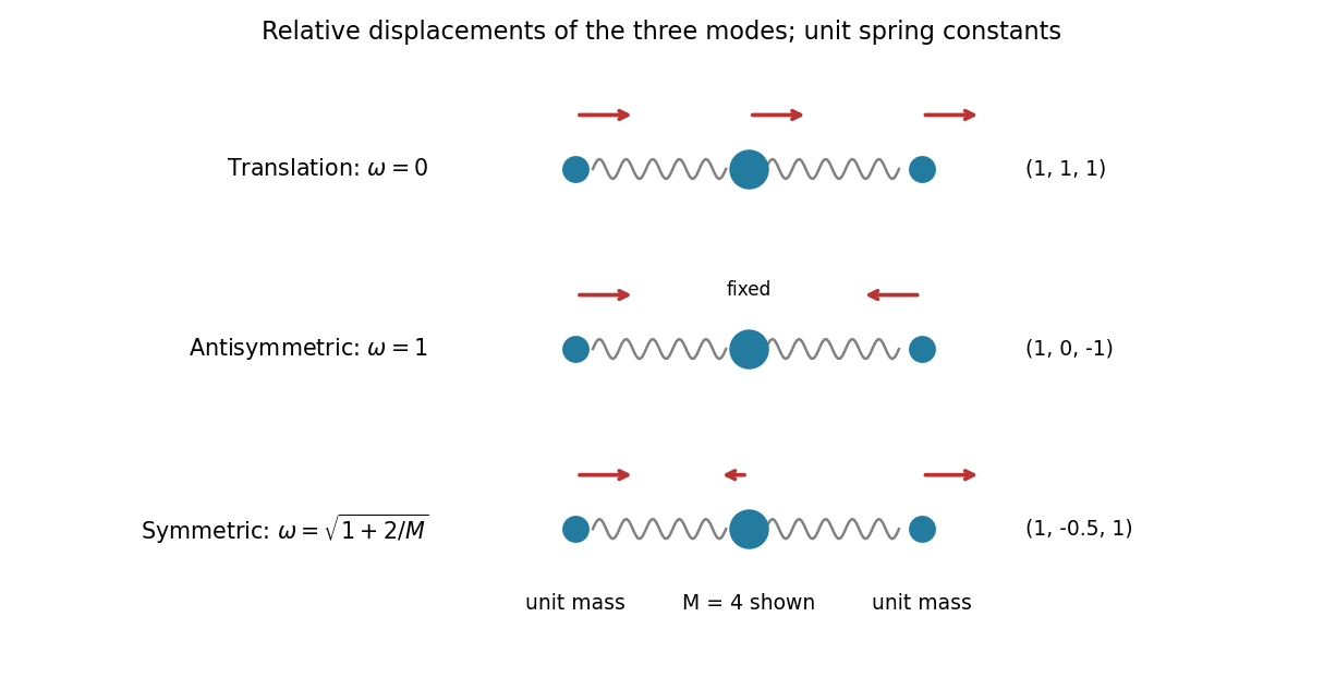
Measure the three coordinates as displacements from a configuration with both springs unstretched. The kinetic energy is , and the potential energy is . Expansion givesFor , direct substitution yields the three normal modes:The three vectors are independent and orthogonal in the mass inner product , so they exhaust the motion. Their squared mass norms are ; division by the corresponding square roots gives normalized modes. This is the unit-spring, unit-outer-mass case of the normal modes of three masses connected by two equal springs.
As , the central displacement in the symmetric oscillatory mode tends to zero and both nonzero frequencies tend to one. The two limiting shapes and span independent motions of the outer masses against an effectively fixed centre; each unit mass has its own unit spring frequency. The translational mode remains at zero frequency. Under a bounded kinetic-energy condition its common velocity tends to zero as , while a static common displacement is still an equilibrium shift. One must specify that energy condition before concluding that an arbitrary freely translating heavy mass remains stationary.


A group homomorphism preserves multiplication: . Its group kernel is a subgroup, and for . Thus , proving it is a normal subgroup. The map is well-defined because two representatives of a coset differ by an element of . It is a homomorphism, has trivial kernel, and is surjective when is. This proves the first isomorphism theorem, . This proof does not use finiteness and therefore also applies below.
The identity matrix belongs to . The determinant is multiplicative, giving closure, and matrix multiplication is associative. The inverse of a determinant-one matrix is , also of determinant one. Thus this special linear group is a group.
The fractional linear maps must be interpreted on the Riemann sphere, including infinity: a finite pole is sent to infinity and infinity is sent to when . As literal everywhere-defined maps of the complex plane they would not form the asserted group. Substitution into the two rational expressions gives . Matrix identities and inverses therefore give the identity and inverse transformations, proving that the Möbius group is a group and that is a surjective homomorphism.
For to be the identity, on all finite points where defined. Hence is the zero polynomial, so , , and from the determinant. ThereforeThe kernel is central and hence normal. In particular is not an isomorphism, since and represent the same transformation. The quotient is the projective special linear group in this complex two-dimensional case.
For a subgroup of a finite group , distinct left cosets are disjoint and partition . Each coset has exactly elements because is a bijection. Counting the partition proves Lagrange's theorem:A cyclic group is generated by a single element. In a group of order four, an element of order four generates the whole group, giving . Otherwise all three nonidentity elements have order two. Choose two of them ; cancellation makes the third. Since , . The remaining products then give the Klein four-group. This proves that there are precisely two groups of order four up to isomorphism, distinguished by whether an element of order four exists.
For the square, take to be counterclockwise rotation by and reflection in the horizontal axis. They satisfy and . The dihedral group here is of order eight, with elements . Both generators are necessary: one generator would give a cyclic, hence abelian, group, while and do not commute. In the following Cayley table, the row acts after the column; the formula , with exponents reduced modulo four and two, computes every entry.The largest cyclic subgroup is , of order four. Every reflection has order two and there is no element of order eight. The other subgroups of order four areBoth are Klein four-groups, generated by the commuting involutions and one reflection. For completeness, any order-four subgroup containing or equals . Otherwise it contains a reflection ; the product of two distinct reflections is a nonidentity rotation, which must be if odd powers of are excluded. This forces the subgroup to be , giving exactly the two displayed choices. It is the square case of the classification of subgroups of a dihedral group.
The Klein four-group has multiplication tableSince it is abelian, every conjugacy class is a singleton: . An irreducible representation is a nonzero representation whose only invariant subspaces are zero and the whole representation space. For a finite group, the number of inequivalent complex irreducible representations equals the number of conjugacy classes, so there are four here.
A one-dimensional representation sends the involutions to signs, independently. All four choices areThey are distinct irreducible representations, exhausting the four possibilities. The character table of the Klein four-group isThe specified diagonal matrices obey , commute, and satisfy , so the group relations prove that is a group representation. Its coordinate axes are invariant lines carrying respectively . ThereforeThe trivial representation is absent. If denotes the four-row character matrix above, direct row products give . This verifies character orthogonality:The character of is , whose inner products with the four rows are , independently confirming the decomposition. All these irreducibles are real as well: commuting real involutions can be simultaneously diagonalized into their real sign eigenspaces.
Articles by others on the same topic
There are currently no matching articles.