Use the unitary position-to-momentum Fourier transform . Integration giveswhere with its continuous value one at zero. The amplitude is real and even, with central maximum , zeros at for nonzero integer , and alternating-sign sidelobes decaying as .
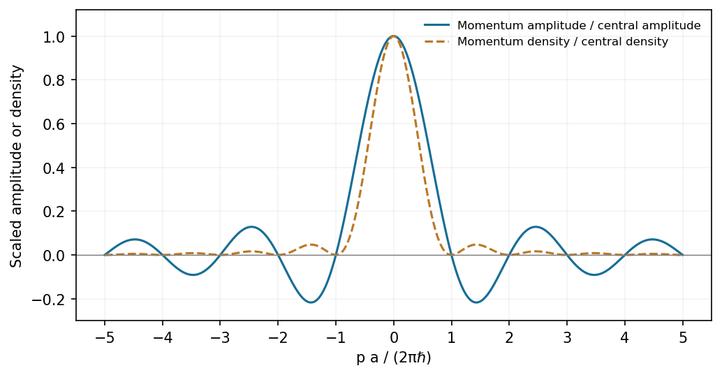
A finite rectangular position amplitude gives a sinc momentum amplitude and a sinc-squared momentum density
. Source. Details. 
The probability density is , not the signed Sinc function amplitude. Its integral is one by the unitarity of the Fourier transform.
Nonrelativistic acceleration from rest gives and . The observed deflection is the angle between incident and diffracted beams, , so Bragg's law at first order givesHere . The numerical evaluation uses the externally documented CODATA 2014 values , and ; it does not assert which rounded constants were in the exam's handbook. Relativistic corrections at this voltage are negligible at the precision of the angle.[ref]
If , the Hermitian operator property makes real. Applying the operator identity to this eigenvector gives . Its only real root is ; the other cube roots of unity are nonreal. In an orthonormal eigenbasis, . Equivalently, the spectral theorem places the entire spectrum of the self-adjoint observable at one, giving the same conclusion. The quantum-mechanical setting assumes the usual well-defined observable and operator domains.
At the central values, . For independent input standard errors, linear propagation givesThe angular derivative here is with respect to radians, so . At , the derivative is one, andThus , with the stated measurement uncertainty interpreted as one standard error. Correlated inputs would require a covariance term; their correlation is not supplied.
For independent charge arrivals described by a Poisson distribution, the one-sided Shot noise current Power spectral density is . Treating the stated bandwidth as the Effective noise bandwidth,The expected rms noise is , about of the mean current. This is the full Shot noise value with Fano factor one; correlations can suppress or enhance it. The elementary charge is from the external CODATA 2014 table.[ref]
For the oppositely travelling components, write and after removing the common time phase. Then . In the interference terms contribute no imaginary part, soA standing-wave interference pattern can therefore change density without adding a cross-term to the net current.
For barrier-top scattering, the stationary equation inside the barrier is . Thus its spatial part is linear: . Take incident amplitude one, and . Continuity of the spatial wave function and its derivative at the two finite steps givesSolving these four equations yieldsThe equal exterior velocities mean flux ratios are squared amplitude ratios:This is the threshold limit of finite-barrier scattering, not exponential decay with a nonzero interior decay constant.
The interior constants areSince ,It is positive and independent of position, matching the transmitted flux. Although the classical kinetic energy inside is zero, the complex linear quantum wave function carries conserved probability current; its phase varies with position.
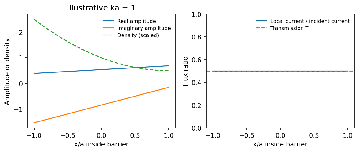
At the barrier-top energy the complex amplitude is linear while its probability current remains constant
. Source. Details. 
Differentiating the expectation value and using and givesThe second term means explicit operator time dependence, distinct from the state's evolution.
The commutator product rule follows by adding and subtracting :For the mathematical induction step, let and use . The case is immediate. If , thenThus the claimed identity holds for every positive integer. Commutation of with is not needed for this particular step. This is the central-commutator differentiation rule. Termwise application to a convergent power series, on a common domain where the operations are justified, gives
For position and momentum, . Hence , and . Substitution gives Ehrenfest theorem:The mean momentum changes by the mean force. It does not follow for a general nonlinear Potential energy that : a closed classical trajectory for the mean position requires an additional condition, such as a quadratic Potential energy or a sufficiently localized wave packet.
Expanding with the angular momentum commutators givesFor , commuting past a ladder operator givesThus the raised or lowered vector, if nonzero, is an eigenvector with the shifted eigenvalue; an angular momentum ladder endpoint can instead be annihilated. Also , so for every nonzero ladder result.
For orbital angular momentum, gives an azimuthal factor . Single-valuedness under requires integer . Positivity of ladder norms givesfor normalized states. A fixed finite therefore has upper and lower endpoints. Writing the upper endpoint as , its vanishing raising norm gives ; the lower endpoint is . Consequentlywith . This integer conclusion is for orbital angular momentum; spin representations can also have half-integer labels.
For the specified Gaussian-radial state, use a Cartesian p-orbital decomposition: write . Its angular factor isOnly occurs. The squared angular coefficients are before common normalization, so each allowed has probability one third. Therefore the simultaneous outcome isThe common normalized radial factor cancels from this ratio. The standard symmetric sequence used above resolves the duplicated central positive entry in the printed list.
Direct matrix multiplication givesThe normalized eigenvectors are , and the eigenvectors are , with eigenvalues in each case.
For , allowing for a possibly unnormalized input pair of coefficients,For a normalized state . The second result follows because each squared Spin operator matrix equals .
The tilted component is . Its eigenvalues remain , with one real phase convention for the normalized eigenvectorsProjecting the initial onto them gives and . ThusA smaller expectation does not imply a smaller individual spin eigenvalue; it describes the probabilities of the same two measurement outcomes.
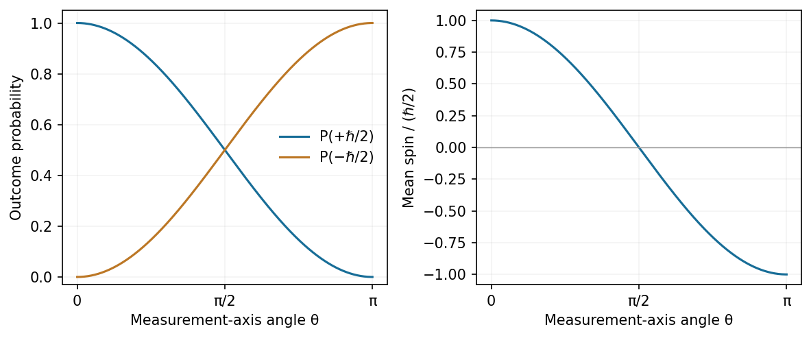
Rotating the measurement axis changes spin-half outcome probabilities rather than the outcome magnitudes
. Source. Details. 
identical particles have the same intrinsic properties, including mass, charge and spin. Their labels are bookkeeping devices rather than measurable identities. When wave functions overlap, quantum mechanics supplies no observable trajectory that permanently identifies “particle 1” independently of “particle 2”. A many-particle description must therefore treat exchange consistently. The Hamiltonian and physical observables are invariant under relabelling identical particles.
For two particles, the exchange operator obeys . The usual three-dimensional symmetrization postulate selects states symmetric under exchange for bosons and antisymmetric for fermions. In relativistic quantum theory, the Spin-statistics theorem associates integer spin with bosons and half-integer spin with fermions under its locality and positivity assumptions; the connection is not derived merely from in elementary nonrelativistic mechanics. For orthonormal one-particle states and , the two-particle spatial combinations areThe sign concerns the complete state, including spin and other internal variables, not necessarily the spatial factor alone.
The antisymmetric state vanishes if both fermions occupy the same one-particle state: this is the Pauli exclusion principle. For fermions in orthonormal spin orbitals , the normalized Slater determinant supplies the required exchange sign. Bosonic occupation has no corresponding upper limit, and symmetrized products describe many bosons. Fermionic occupation is zero or one per complete one-particle state; two electrons can still occupy the same spatial atomic orbital with opposite spin.
Spin and spatial symmetry are linked. A two-electron spin singlet state is antisymmetric, so its spatial factor must be symmetric. A symmetric triplet state instead requires an antisymmetric spatial factor. Exchange then changes pair correlations and the energies available when interactions depend on particle separation, even without introducing a new classical “exchange force”. It contributes to atomic shell structure, bonding and magnetic behaviour.
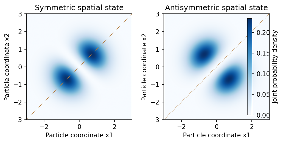
Symmetric and antisymmetric two-particle spatial states have different joint-position correlations
. Source. Details. 
In an occupation-number description, bosonic creation and annihilation operators satisfy , whereas fermionic operators satisfy and anticommute among themselves. The latter imply . This formalism implements the same exchange constraints without assigning permanent particle labels.
For noninteracting particles in thermal equilibrium, the mean occupation of a state of energy isFermi-Dirac statistics produces a filled Fermi sea at zero temperature and degeneracy pressure; Bose-Einstein statistics permits macroscopic Ground state occupation when the density of available states and thermodynamic conditions allow condensation. The different statistics therefore have measurable collective consequences, not just different notation.[ref]
Statistical Physics by David Tong. Chapter 3, §§3.5–3.6: Bose and Fermi distributions, condensation and degenerate Fermi gases
When phase-space occupation is dilute, both distributions reduce to the Maxwell–Boltzmann statistics limit. Likewise, well-separated localized wave packets have negligible overlap and small exchange corrections, so effectively labelled classical trajectories can become a useful approximation. In two spatial dimensions more general exchange statistics are possible; the standard boson/fermion account here concerns ordinary three-dimensional particles and their total states.
For the nonrelativistic Coulomb Hamiltonian with reduced electron-proton mass , separation in Spherical coordinate system gives . The quantum numbers obey , and . These are joint eigenstates of energy, and , with the latter two eigenvalues and .
The Coulomb bound-state energies and characteristic length areFor example, is spherically symmetric and has no radial node. In general the radial part contains an exponential times a Generalized Laguerre polynomial, with radial nodes. The spherical harmonic specifies angular structure and azimuthal phase; real linear combinations of degenerate states give familiar directional orbitals.
The leading Coulomb energy depends on alone, giving spatial states for each principal shell, or including electron spin. Fine structure, Lamb shift and Hyperfine structure lift parts of this ideal degeneracy. An atomic orbital is a probability amplitude, not a classical planetary path.[ref]
Quantum tunnelling is supported by transport and decay through barriers that classical particles of the same energy cannot traverse. Three complementary examples are:
- In alpha decay, an alpha cluster escapes the attractive nuclear region through a Coulomb barrier. The barrier penetration factor depends exponentially on a forbidden-region action, helping explain the strong dependence of lifetimes on emitted alpha energy. This is evidence from systematic decay rates, rather than direct imaging of an alpha inside the barrier.
- A scanning tunnelling microscope measures current across a narrow vacuum gap between a conducting tip and sample. At small bias an approximate dependence is with . The strong gap-distance sensitivity enables atomic-scale imaging and local spectroscopy. Electronic density of states and barrier height also affect the current, so constant-current contrast is not an unqualified geometric atom map.[ref]Surface Studies by Scanning Tunneling Microscopy by Gerd Binnig and others. Vacuum-tunnelling measurement and surface imaging
- A heavily doped Tunnel diode has a narrow p-n barrier. Bias changes the overlap of occupied and empty states across it; interband tunnelling produces a characteristic peak and Negative differential resistance interval in its current-voltage curve. The measured voltage dependence agrees with the changing band overlap, providing a solid-state transport example.[ref]New Phenomenon in Narrow Germanium Junctions by Leo Esaki. Germanium-junction tunnelling characteristic
Together these test barrier penetration in nuclear decay, vacuum-gap transport and semiconductor transport. Their detailed currents depend on state supply and matching as well as the barrier transmission probability.
For the Quantum harmonic oscillator defineThe Canonical commutation relation gives , andThus the creation operator and annihilation operator raise or lower the energy by one quantum. Positivity of and termination of downward stepping give , . Normalized actions are and . The annihilated ground state obeysThe nonzero Ground state energy is the zero-point energy, consistent with position-momentum quantum uncertainty. Since , a perturbation linear in position connects only neighbouring number states. The algebra is especially useful for matrix elements and selection rules.[ref]
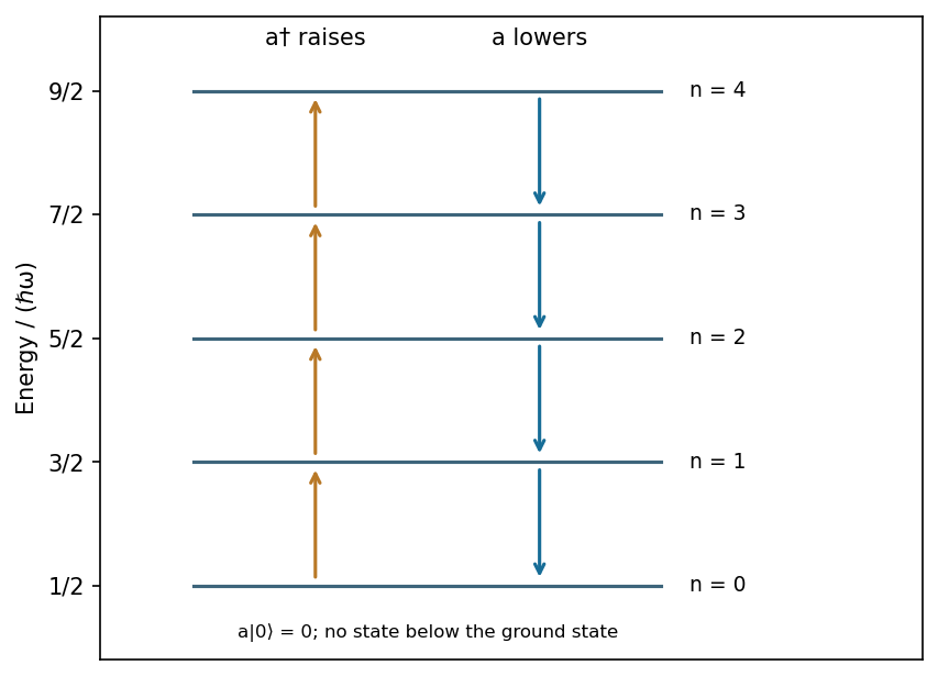
Creation and annihilation connect equally spaced oscillator levels while the ground-state lowering action vanishes
. Source. Details. 
The ideal voltage-feedback Operational amplifier has zero input currents and, while stable negative feedback holds it in its linear operating range, equal input voltages: and . The first rule follows from infinite input impedance; the second is the large-open-loop-gain limit of . Equal input electric potential is a virtual short, not an electrically conducting connection.
For an inverting amplifier with the noninverting input grounded, and node-current balance gives , hence . For a noninverting amplifier, the feedback divider gives , hence .
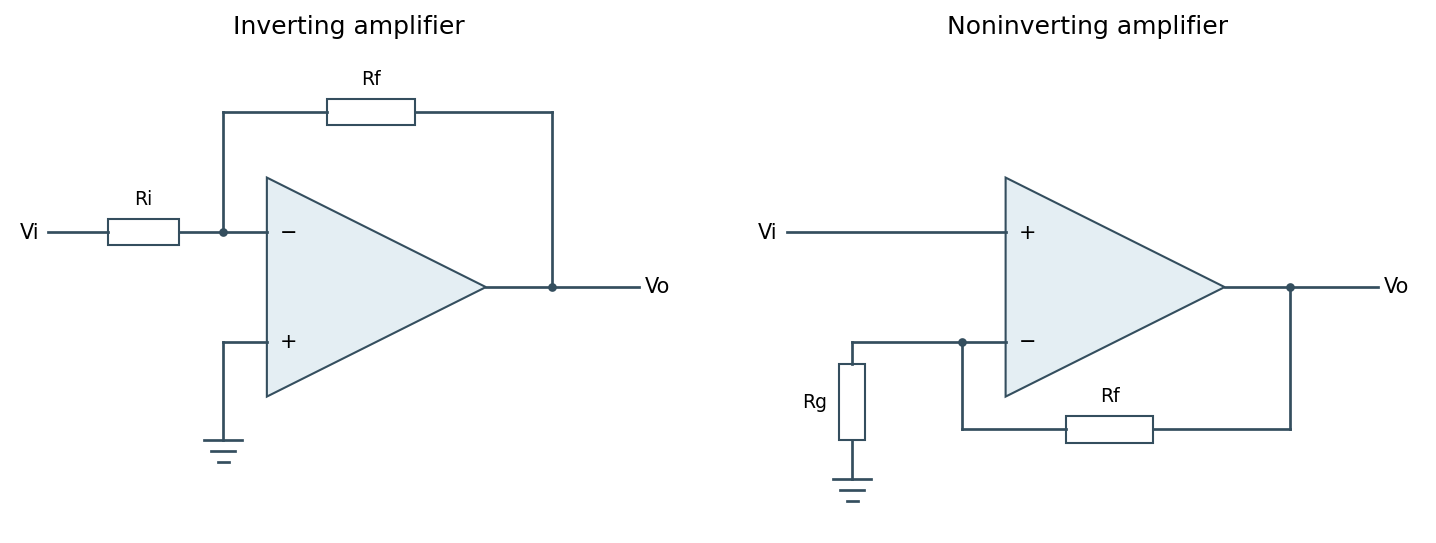
Ideal inverting and noninverting negative-feedback configurations
. Source. Details. 
One should check output swing, input common-mode range, slew rate, Gain-bandwidth product and stability before using these limits in a real circuit. Saturation, positive feedback or operation beyond bandwidth invalidates the equal-voltage rule; finite input bias currents and offset voltage can also matter.[ref]
Operational-amplifier negative feedback by Analog Devices. University electronics course, Chapter 3: high-gain feedback assumptions and practical limits
Thermal agitation in a resistor produces Johnson-Nyquist noise, even without an applied mean current. In the classical low-frequency regime, its one-sided open-circuit voltage spectrum is and its equivalent short-circuit current spectrum is . In an Effective noise bandwidth ,For a matched load, available thermal noise power is . A resistor and load at the same temperature exchange noise power without a net heat flow.
Cooling reduces the rms amplitude as if Electrical resistance and bandwidth remain fixed. A cryogenic bath or refrigerator, thermal anchoring and controlled heat input can maintain a steady low temperature. Radiation shields, an insulating vacuum, thermally anchored leads and limited measurement dissipation reduce heat leaks and self-heating. Temperature sensing and stable feedback control reduce slow temperature-induced drift; keeping temperature constant does not remove microscopic thermal fluctuations.
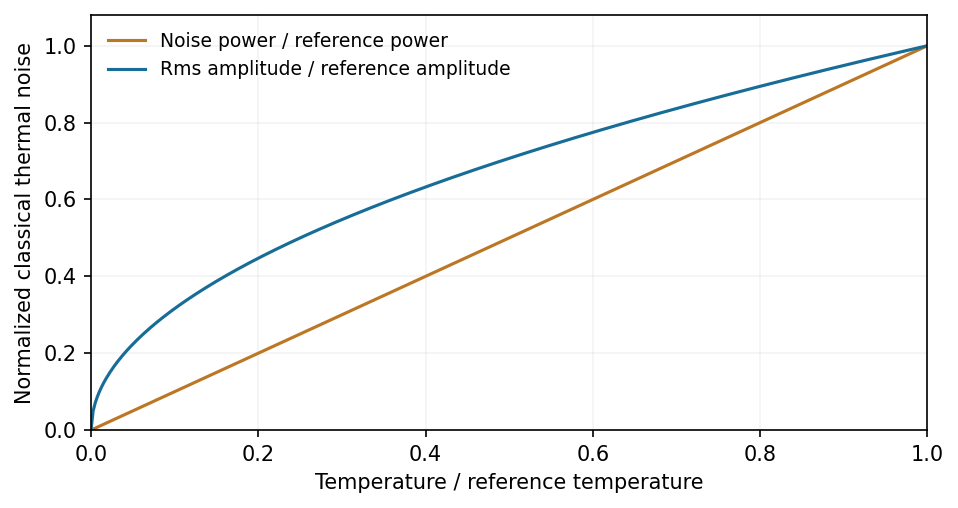
At fixed resistance and bandwidth, thermal-noise power scales with temperature and rms amplitude with its square root
. Source. Details. 
Bandwidth restriction, suitable impedance and a low-noise amplifier complement cooling. Warm leads, contacts and the amplifier can otherwise dominate the observed noise. At fixed mean current, shot noise is not generally reduced merely by cooling, and low-frequency excess noise need not follow the Johnson law. At frequencies with , quantum noise expressions replace the classical approximation.[ref]
Op-amp Noise by Analog Devices. Distinction between resistor thermal noise, amplifier noise and current-noise contributions
Uniform signal sampling at rate multiplies a continuous signal by a time-domain Dirac comb, giving frequency-domain replicas spaced by :If a baseband signal is restricted to and , these replicas can be separated by an ideal reconstruction filter. Frequencies differing by integer multiples of have the same sampled phase progression; for real signals they fold into the interval from zero to . This ambiguity is aliasing.
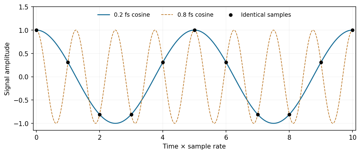
Two different continuous cosine frequencies produce the same samples when one lies above Nyquist
. Source. Details. 
For example, and cosines produce identical sample values. Apply an analogue Anti-aliasing filter before digitization and choose enough sample-rate margin for its finite transition band. A digital filter applied afterward cannot distinguish components already folded onto one another. Out-of-band noise also aliases unless filtered. The sample rate sets temporal/spectral coverage; quantization resolution sets amplitude precision and is a separate limitation. Bandpass Signal sampling has additional conditions beyond the simple baseband rule.[ref]
What the Nyquist Criterion Means to Your Sampled Data System Design by Walt Kester. MT-002: spectral replicas, aliases and practical filtering
Articles by others on the same topic
There are currently no matching articles.