Use arc length as the affine parameter, and put a dot over derivatives with respect to . The geodesic Lagrangian on the sphere isThe cyclic coordinate gives . With the constant normalized as in the paper,Here has units of inverse length, because is physical arc length. Unit-speed normalization givesFor , division by yields the spherical-geodesic first integralThe turning latitudes satisfy . In the usual polar-coordinate range ,The maximum departure from the equator, often the geometric quantity intended by an angular amplitude, is insteadThus polar angle and signed latitude must not be interchanged. At the geodesic is the equator. At it is a meridian through the poles; cannot serve as a global parameter and the divided equation is inapplicable. The limiting polar range is then .
The original PDF prints an ambiguous derivative with the square on rather than a conventional derivative notation. If the intended equation was second order, differentiating the first integral, or eliminating from the Euler-Lagrange equation, gives the equally useful formIt has the same normalized geodesics and the same turning angles. Giving both forms resolves the typographical ambiguity without pretending that a second derivative is the square of a first derivative. Geometrically these trajectories are great circles, with inclination to the equator.
Assume an emitter at rest on the stellar surface and a static observer at infinity. Write . The time-translation Killing energy of a photon is conserved, while the locally measured photon energy is proportional to . ConsequentlyUsing , , and ,The Schwarzschild radius is approximately , below the given surface radius. The positive shift is therefore a gravitational redshift of an escaping photon, with received wavelength about times the emitted wavelength. A moving emitter would introduce an additional Doppler factor; that is outside this static-surface model. The weak-field estimate is insufficient at this compactness. These stated constants are numerical conventions, not a claim about an unavailable historical handbook's last digits.
Use metric signature and four-velocities , with . Their Lorentz invariant inner product isIn the rest frame of either particle this same scalar is the relative Lorentz factor . HenceLet . The numerator after combining terms isUse to obtainThe two rest frames agree on the relative speed, although their velocity vectors are expressed in different spatial frames. Checks include equal velocities giving zero, collinear velocities giving , and low speeds reducing to the Galilean relative speed. For timelike particles the four-velocity inner product also ensures .
A tidal force is a difference of gravitational acceleration across an extended region. In Newtonian gravity, . Two neighboring freely falling particles separated by have, to first order,For a point mass, . In a local orthonormal radial/transverse frame,A small freely falling cloud stretches radially and compresses transversely. Outside the source the three eigenvalues sum to zero, consistently with ; within matter the trace is . These are accelerations of separations, not the much larger common acceleration of the cloud's centre.
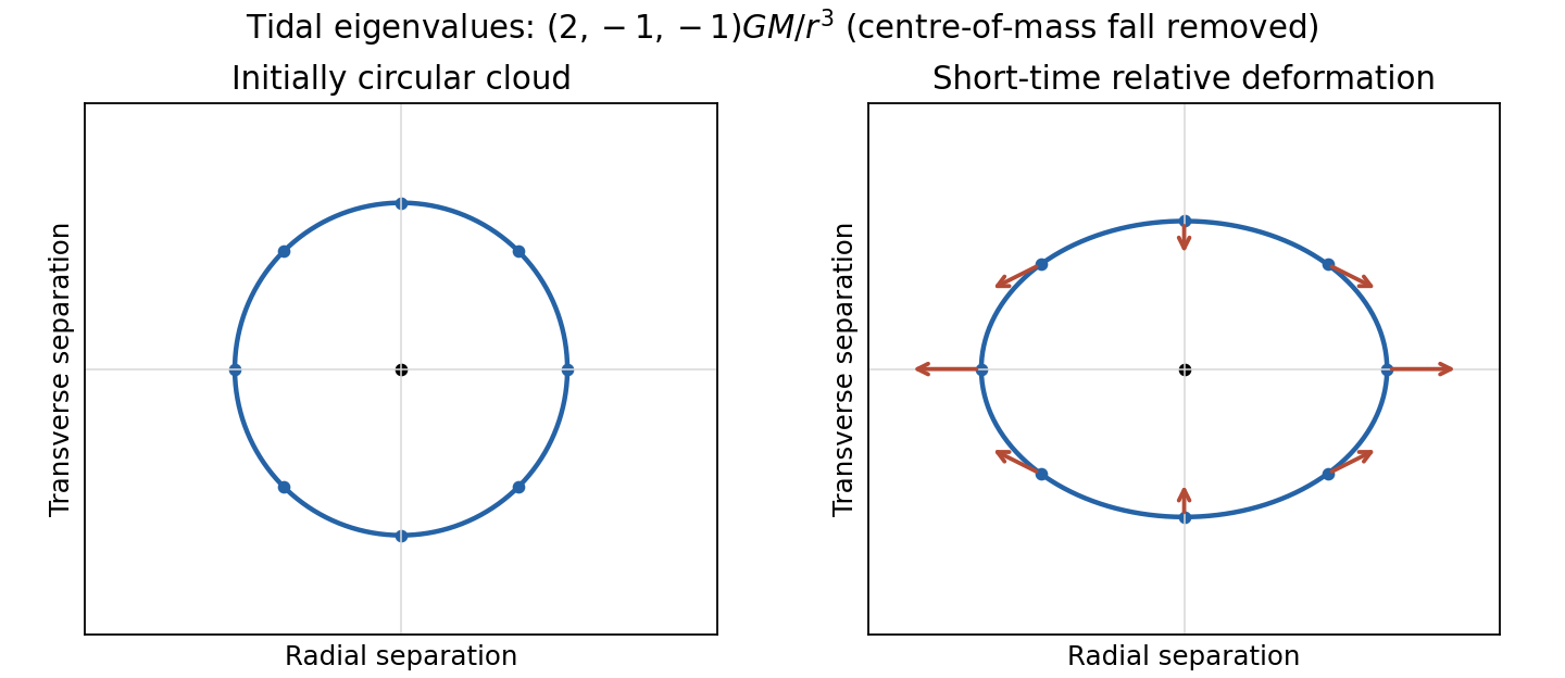
Original local tidal map: a freely falling cloud stretches along the radial direction and contracts in both transverse directions
. Details. 
In general relativity, freely falling test particles follow timelike geodesics. A freely falling frame can eliminate the connection at one event, but not the Riemann curvature tensor throughout a finite laboratory. Let be the geodesic tangent and a connecting vector for neighboring geodesics with . In the explicitly chosen curvature conventionthe geodesic deviation equation isIt follows by commuting , using and zero torsion. In a parallel-propagated orthonormal frame, its spatial components directly describe measured relative acceleration. The weak-field, slow-motion limit recovers the Newtonian Hessian above. Reversing the curvature sign convention reverses the displayed curvature side, without changing the physical stretching. The equivalence principle removes locally uniform gravity, while geodesic deviation measures the residual tidal field. The connection between parallel transport, curvature and neighboring geodesics is developed systematically in the standard geometric construction.[ref]
Lecture Notes on General Relativity by Sean M. Carroll. Section 3, Curvature: parallel transport and geodesic deviation; translate the chosen curvature sign consistently
The cosmological principle idealizes spatial slices as homogeneous and isotropic. The corresponding Friedmann-Lemaître-Robertson-Walker metric can be writtenHere is cosmic time, has dimensions of length in this convention, and is a dimensionless comoving coordinate. The sign of gives positive, zero or negative spatial curvature. It does not alone determine global topology. A comoving pair at fixed radial coordinates has proper separation scaling with , so the Hubble parameter is , and cosmological redshift satisfies .
For a perfect fluid of mass-equivalent energy density and pressure , Einstein's equations giveThe last equation is local energy conservation for constant , with vacuum energy kept separate from . A component with has : pressureless matter dilutes as and radiation as , the additional radiation factor being photon redshift. With , matter domination gives and radiation domination gives . Positive vacuum energy alone gives exponential expansion, with .
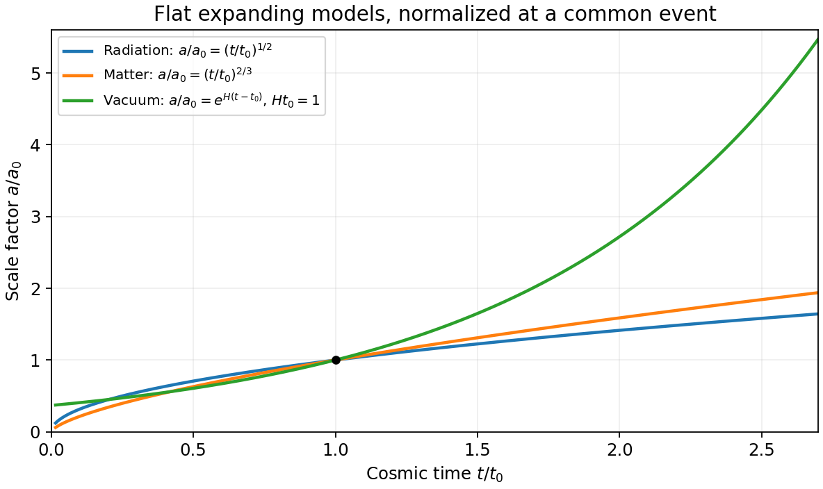
Original comparison of normalized scale factors in flat radiation, matter and positive-vacuum models; the vacuum model has no finite-time big-bang origin in this chart
. Details. 
Geometry, contents and initial conditions together determine the expansion history. A closed matter-only model recollapses; an open matter-only model expands indefinitely. With a cosmological constant, positive spatial curvature no longer by itself implies recollapse. Present critical density is and the density parameters obey , where . These models describe the large-scale background, while local structure and inhomogeneities require perturbations or more general metrics.
Ordinary component differences at neighboring points depend on how the local bases vary. The covariant derivative corrects for that variation:Each upper tensor index adds a connection term and each lower index subtracts one. A scalar has , while the derivative of a tensor transforms as a tensor with one additional covariant index. The Christoffel symbols themselves are not tensor components; their inhomogeneous transformation cancels that of the ordinary derivative.
For the Levi-Civita connection,These express metric compatibility and zero torsion. Along , parallel transport is the initial value problemIt preserves inner products for the Levi-Civita connection. Parallel transport of the tangent itself gives the affinely parametrized geodesic equation, .
Transport generally depends on the path. On a round sphere, transport a tangent vector around the triangle bounded by two meridians degrees apart and the intervening equatorial arc. All three sides are geodesics; the enclosed spherical area is . The returning vector is rotated by degrees, with sign set by traversal orientation. Locally this holonomy is controlled by curvature, even though the connection can be made zero at a single point. A vector can therefore have changing coordinate components while remaining parallel, and constant components do not generally mean parallel transport.
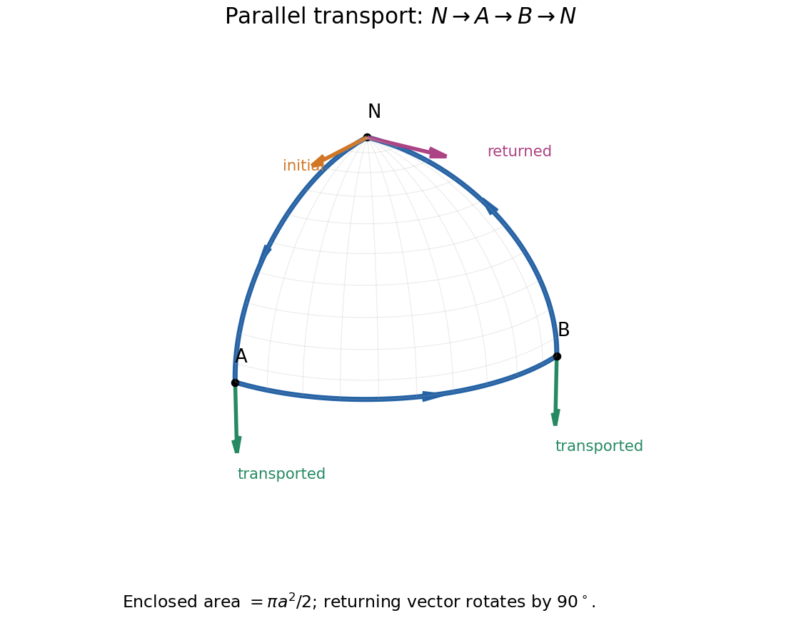
Original spherical-triangle transport: a tangent initially pointing along the first meridian returns rotated by ninety degrees
. Details. 
This construction compares directions at separate points through a chosen connection, rather than assuming that a curved manifold supplies a path-independent comparison.[ref]
Use Cartesian coordinates with and . Spatial dot and cross products below use the Euclidean three-metric. The alternating tensor is given the orientation .
Vector and covector transformation. The vector is independent of coordinates, and the chain rule gives . Likewise the one-form is independent of coordinates. Comparing coefficients provesTheir contraction is unchanged because the forward and inverse Jacobians cancel. Here lowering an index uses the metric, not an identification of the numerical upper and lower components.
Why antisymmetrization matters. Write . Differentiating the covector law givesThe last term obstructs the general tensor transformation law. It is symmetric in , so it cancels from . ThereforeEquivalently is the exterior derivative of the electromagnetic four-potential one-form. The statement that is not a tensor needs a qualification: under affine Cartesian Lorentz transformations it does transform tensorially, because the second derivatives vanish. The failure concerns arbitrary nonlinear coordinate changes, including curvilinear coordinates in flat spacetime. This distinction is precisely the difference between general covariance and covariance under the restricted inertial-frame transformations.[ref]
Lecture Notes on General Relativity by Sean M. Carroll. Section 2, Manifolds, equations 2.26–2.27: the extra second-derivative term and its cancellation under antisymmetrization
Electric and magnetic components. Choose , so , and . ThenThus the lower-index field tensor isThis is a derived component representation of the field, with the source's sign convention.
Raised indices and the first invariant. Raising both indices changes the time-space signs and leaves the spatial block unchanged:In the scalar contraction, each independent antisymmetric pair is counted twice, givingUnder a Lorentz transformation each inverse transformation from a lower index cancels its matching transformation from an upper index, leaving the same scalar. In particular a plane electromagnetic wave has in these units and makes this invariant vanish, while a pure electric field makes it negative.
The printed dual convention. The PDF explicitly defines , with no . Each independent pair therefore contributes twice: for example . The complete result isThe time-space pairs contribute and the spatial pairs contribute another . The conventional Hodge dual includes and would instead give the contraction ; it must not silently replace this paper's definition. With fixed orientation the latter contraction is a pseudoscalar: invariant under proper Lorentz transformations but odd under orientation reversal if compared using a fixed alternating symbol.
Energy density and flux. Substitution into the given mixed stress-energy tensor yieldsFor the first formula, and . For the second, . The minus sign on arises from its lowered spatial index; it does not reverse the physical energy flow. Raising that index gives , and symmetry gives , with the Poynting vector in units. Thus is energy density and represents energy flux. In SI coordinates , restore and , with . This keeps the mixed-index signs and the units distinct.
Put , where , and work in the orbital plane. A dot denotes an affine-parameter derivative; for a material particle choose that parameter to be proper time.
First integrals and normalization. The geodesic Lagrangian isTime translation and axial rotation make and cyclic, givingThe tangent norm is constant along an affine geodesic because the Levi-Civita connection preserves the metric. ThereforeFor proper-time parametrization of a timelike worldline this norm is . For a null geodesic it is zero, for every affine normalization. Thus for the chosen material-particle normalization and for light. Proper time cannot itself parametrize a null ray, despite the same printed symbol being used for its affine parameter.
Null normalization and impact parameter. Under with , both and scale as , while the null path is unchanged. Their ratio is invariant. At large radius the spatial speed with respect to asymptotic time is , and orbital angular momentum per affine tangent givesFor an orientation chosen with , this is . Setting is a choice of affine scale, not a claim that all photons have equal measured energy. Once a tangent is identified with a physically normalized four-momentum, its energy fixes that scale.
Orbit shape. Substituting the constants in the norm and multiplying by givesFor and , . HenceThe radial orbit must be treated with the radial equation, because azimuth is then constant.
Circular photons and stability. For a null ray define . Its radial equation becomesThe circular orbit requires and , soIt is at a maximum of the null effective potential and is unstable. Equivalently the Binet equation linearizes about to , admitting exponentially growing radial deviations in azimuth.
Capture from infinity. Divide the null radial equation by . The quantity opposing inward motion is , whose exterior maximum is . There is no outer radial turning point precisely whenAt equality an exactly critical ray from infinity asymptotes to the photon sphere; it does not cross the horizon at a finite affine parameter. Above the threshold an initially inward ray from infinity reaches an outer turning point and scatters. The radial case is also captured. These statements refer to inward rays launched from the asymptotically flat exterior, not arbitrary initial data inside the angular-momentum barrier.
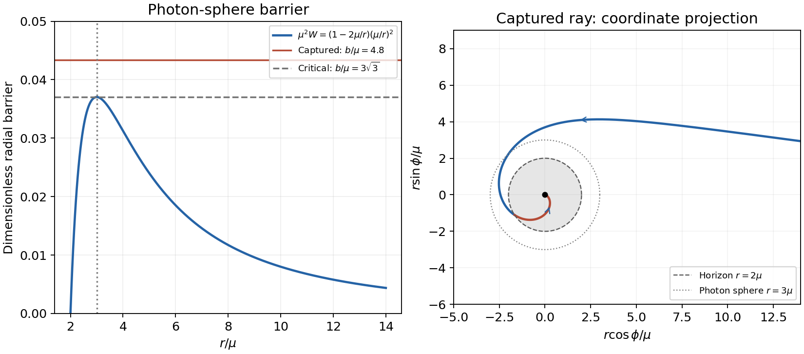
Original Schwarzschild capture calculation: the null-potential barrier and a captured equatorial ray crossing the horizon and ending at finite azimuth
. Details. 
Approach to the singularity. A captured nonradial ray bends inward, crosses and then the event horizon , and continues toward the curvature singularity. A plot in is only a coordinate projection, not a Euclidean spatial slice inside the horizon. For large the cubic term in the shape equation dominates:for the inward branch with . Its integral isThus the azimuth tends to a finite limit at the singularity, rather than winding infinitely often there. Near-critical rays can accumulate many turns near before capture, which is a separate phenomenon. A strictly radial ray has constant azimuth and does not admit this azimuthal asymptotic form. The radial equation also gives for a nonradial null ray, confirming finite remaining affine parameter.
Material capture and the condition at infinity. To recover the quoted threshold, take the usual marginally bound orbit, initially at rest at infinity: . With ,The turning-point quadratic has discriminant . It is positive for large and has no real positive root when , while the radial case also falls in. ThereforeAt equality the quadratic is proportional to and the orbit asymptotes to the unstable marginally bound circular orbit at . For larger , an incoming marginally bound particle encounters the outer turning point and scatters.
The source says only “from infinity”, without explicitly fixing the asymptotic speed. For a general incoming speed , andThe same bound remains sufficient for capture, since the added constant is nonnegative. It is the exact threshold only for . At fixed , the critical unstable orbit satisfiesThen . This states both the printed sufficient condition and the additional assumption needed to call it a sharp capture boundary.
Articles by others on the same topic
There are currently no matching articles.