Write for the cross-sectional area, and use consistently for the longitudinal coordinate: the paper's later is the same coordinate. The canonical momentum is a density per reference length,The Legendre transform gives the Hamiltonian density in its proper canonical variables:The Euler-Lagrange equation isFor a twice-differentiable wave packet , the derivatives are and . Thus the nontrivial packet solves the wave equation whenThe negative sign gives the opposite propagation direction. Here has units , has units , and has units . The result follows from the supplied axial stiffness in the Lagrangian. For a freely contracting thin elastic rod the relevant longitudinal modulus is normally Young's modulus, rather than the bulk modulus; the question's given Lagrangian fixes which coefficient is being used.
Both Noether charges require boundary conditions that admit the stated transformations and no net boundary-current flux. Take a sufficiently localized field on the whole rod, with the weighted integrals below finite. Fixed endpoints at finite positions generally spoil the waveform-dilation symmetry.
The transformation leaves both derivatives unchanged, so the Lagrangian density and action are invariant. For infinitesimal unit field variation, the Noether current for a first-derivative scalar field is the shift current of an elastic rod,Its divergence vanishes by the equation of motion. The charge is the total longitudinal mechanical momentum to this order in the displacement field.
For , put . Each derivative gains a factor , so . Changing integration variables to contributes , proving exact invariance of the full-space action.
Set . At fixed coordinates, with . Since the density is quadratic in derivatives,The variation is a divergence, so subtract its boundary term in the Noether current:Thus the dilatation charge of a one-dimensional elastic wave isAn overall sign change would give the same conservation law. Unlike , this charge has units of action, . Its explicit factor of is balanced by transport of the weighted momentum density; an explicitly time-dependent charge can still be conserved.
For a rightgoing wave packet, put and assume decays sufficiently rapidly. ThenThe shift charge becomesIt is time independent. It vanishes for a localized displacement packet that returns to the same displacement at both ends, but need not vanish for a localized strain pulse joining different asymptotic displacements.
For the dilation charge, substitute :The change of variables removes all time dependence. This charge also need not vanish; choosing an origin at the packet's energy centroid can make it zero. Conservation assumes the integral exists and there is no boundary flux, rather than merely assuming that the energy is finite.
Position-dependent density. The density remains independent of itself, so the shift Noether charge survives with its altered canonical momentum:A prescribed generic function supplies a fixed spatial scale and breaks scale invariance. For the dilation-current candidate with the corresponding and , the scale-breaking sources in derivative field theories giveThus is generally not conserved. Constant density recovers the earlier case; specially scale-invariant profiles and suitably invariant domains would require separate treatment.
Quartic strain. The extra term in again preserves a uniform field shift. Its time momentum is unchanged, while its spatial current becomes . ThereforeThe new Hamiltonian density is . Under waveform dilation, the quartic term scales with rather than , andHence there is no corresponding conserved for nonzero generic , even if the energy in its candidate expression is updated.
Field-dependent quadratic stiffness. In , the term breaks the uniform field shift:when spatial flux vanishes. Thus is not generally conserved. However all terms still contain exactly two derivatives in total, with a field of zero dilation weight. The factor gains no extra power of , so waveform dilation remains an action symmetry. Its charge isHere as before. Relative to the original charge, the energy term changes; the symmetry survives despite the nonlinear field dependence. These statements concern symmetry conservation, separately from any restrictions on parameters needed for positive elastic energy.
Write for cylindrical radius in this question, not the rod's mass density. A charged relativistic particle in a time-independent magnetic field has the charged-particle electromagnetic Lagrangianwith zero electrostatic potential. The cylindrical speed is . Inside a uniform axial field, choose the symmetric magnetic vector potential , . Its cylindrical curl gives . HenceIn a field-free region far from either end one can use , recovering the requested outside expression. The question's is a velocity-dependent generalized potential, not electrostatic potential energy.
There is an important end-field qualification. A finite axial field that jumps to zero with no radial component would violate Gauss's law for magnetism. The consistent near-axis idealisation is the solenoid fringe field from an axisymmetric vector potential, , giving and . The piecewise Lagrangian is its hard-edge limit and retains fringe impulses through the jump in . Those impulses are essential to the focusing calculation.
The azimuth is a cyclic coordinate, so its canonical momentum is conserved:Initially the velocity is parallel to the axis in a field-free region, so . Conservation of canonical angular momentum across a solenoid fringe therefore gives, inside the uniform field,This holds away from the coordinate singularity ; the Cartesian orbit will be smooth there.
Time independence also conserves the energy Hamiltonian,The velocity-linear magnetic term cancels in this Legendre transform. Thus is constant, as expected because a static magnetic Lorentz force does no work. Mechanical angular momentum can change even though and the total speed are conserved.
In a uniform-field region, is cyclic and is constant. Its equation is . The radial Euler-Lagrange equation isso with and ,The radial equation applies on intervals with a regular signed cylindrical-coordinate description; the Cartesian solution handles axis crossings.
In a field-free region, the equations areFor this particle , so and outside, until a coordinate change is needed at an axis crossing.
Axial velocity is constant within each uniform region, but not across the ends. In a smooth fringe,The entrance develops an azimuthal speed while radial velocity remains zero. Conservation of total speed givesForward passage presumes the radicand is positive. The exit fringe changes axial velocity again. Neglecting these small changes is a paraxial approximation, requiring , rather than an exact consequence of cylindrical symmetry.
Set just inside the entrance, , and . The stated continuity gives . Until the first axis crossing,For the full orbit, including any crossings, use the transverse complex coordinate :This helical solenoid trajectory with zero incident angular momentum is a circle of radius about transverse guiding centre , combined with uniform axial motion. Its cyclotron angular frequency is , and its axial pitch per turn is . The speed check is .
The physical radius is . When the cosine changes sign, a nonnegative-radius coordinate adds to ; this is a coordinate change, not a discontinuous turn of the particle. For or , the limit is simply , .
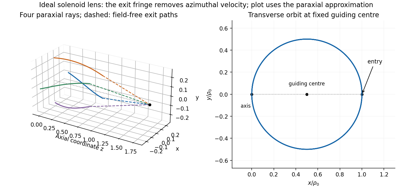
Original solenoid-lens trajectories: transverse circular motion, helical drift and paraxial focusing after the exit fringe
. Details. 
Define the positive focusing frequencyIn the paraxial approximation , traversal time is . The exit values areAcross the exit fringe, and remove the azimuthal velocity. The radial velocity remains continuous in the thin-fringe model. Outside, the transverse trajectory is therefore straight along a fixed azimuth, not a continuing helix. Taking the outgoing axial speed also as , the distance to the axis isIt is independent of , so all equal-speed paraxial rays focus to a common point. The condition ensures the first focus lies beyond the exit. For a weak lens, .
The relativistic solenoid magnetic lens focuses either charge sign, while its rotation reverses with . Keeping the exact radius-dependent , or the exit axial-speed change, produces radius-dependent corrections and spoils an exact common focus. Thus the requested focus is appropriately a paraxial result, with the end fields included even when their axial-speed changes are neglected.
Use metric signature and the model's rescaled units . Its exponential implicitly uses dimensionless rescaled field and coupling combinations; the numerical coefficients of the potential are those supplied. Treat and as independent variables in taking canonical derivatives:The Hamiltonian density isThe kinetic and gradient terms are nonnegative, so a static homogeneous minimum is obtained by minimizing the potential. Put . For , is unbounded below. For , the exponential decays while tends to minus infinity. Thus a stable vacuum requires .
For positive ,The exponential complex-scalar potential consequently hasFor , the minima form a circle , with and . For the minimum has . The symmetry remains global phase rotation in either phase, but a chosen nonzero vacuum breaks it spontaneously. At the origin is a unique minimum with vanishing quadratic curvature and a positive leading quartic term; this critical masslessness should not be confused with a Goldstone mode.
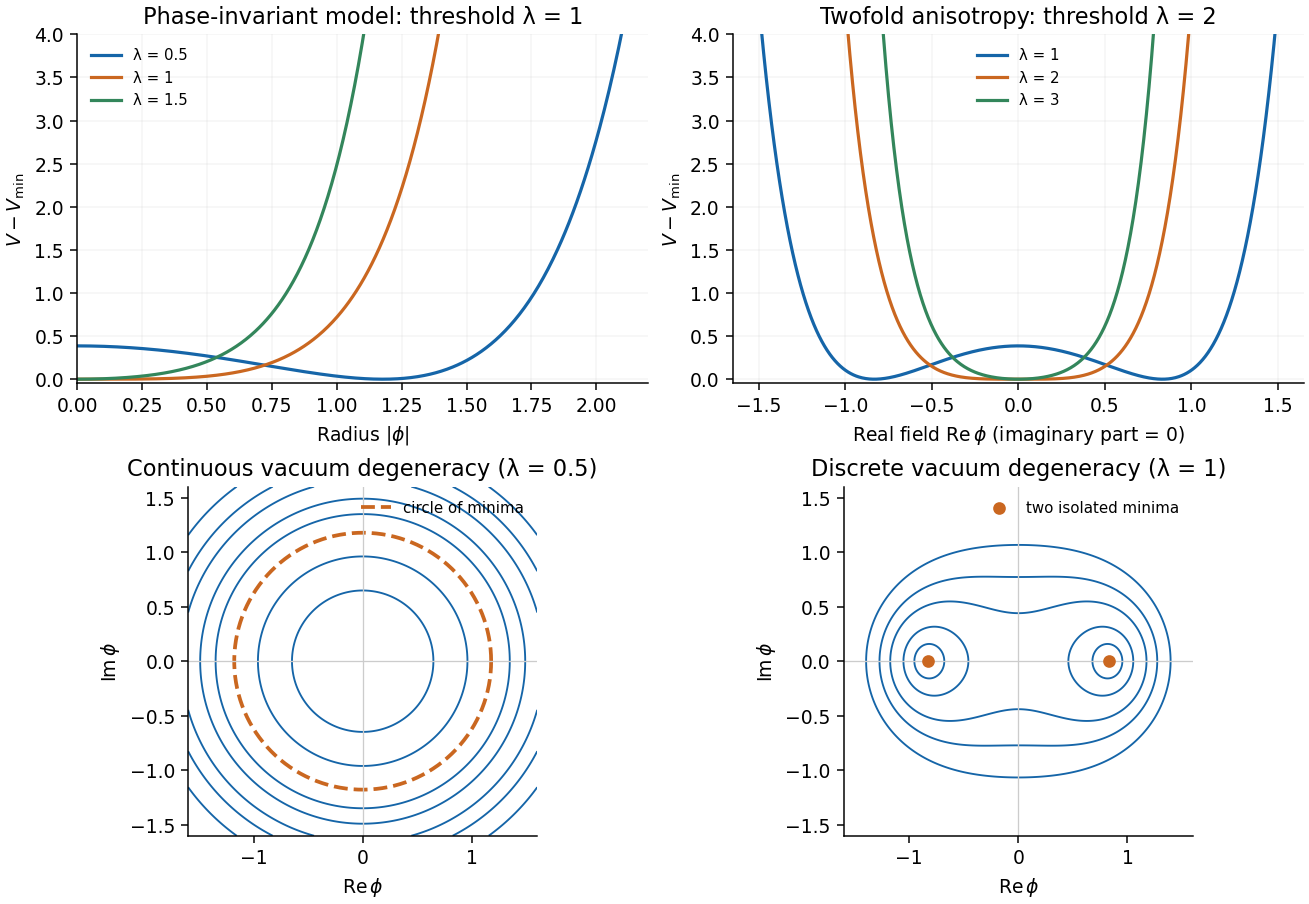
Original radial potentials showing the continuous and explicitly twofold vacuum structures and their thresholds
. Details. 
Let and write . ThenSince and , the quadratic potential isThereforeThe constant can be dropped from the fluctuation equations. For canonical real fields, use :These are the radial and angular masses of a phase-invariant scalar potential. The radial Higgs mode changes the field magnitude and costs energy to second order. The angular Goldstone boson changes the phase along the vacuum circle without a quadratic restoring force. Its linear dispersion is , whereas the radial mode has . The zero angular mass follows the continuous broken global symmetry, not from an accidental cancellation in a particular coordinate choice.
Write . The covariant kinetic term containsA local U(1) gauge symmetry can remove in unitary gauge. The angular fluctuation no longer appears as an independent physical massless Goldstone boson; its degree of freedom supplies the longitudinal polarization of the massive vector field. At quadratic order,The factor of two follows from the convention that is the complex field's vacuum value. This Higgs mechanism changes a two-polarization massless electromagnetic field into a three-polarization massive Proca field; the remaining radial scalar keeps . Static fields in the homogeneous broken phase are screened on a scale of order in these units. The gauge symmetry is a redundancy of the description; the physical statement is the changed spectrum and disappearance of an independent massless angular mode.
Write . The added term is , so the full potential simplifies toThe phase-rotation subgroup is reduced from U(1) to the two-element symmetry . More fully, the kinetic term and potential are invariant under independent reflections and , a internal symmetry generated by and complex conjugation. There is no continuous internal rotation symmetry for the explicit twofold anisotropy of a complex scalar field.
For fixed , positive makes the exponential grow with , so every global minimum has . On the real axis,ThusFor , the nonzero stationary points are the two global minima; the origin is unstable along the real direction. For the origin is the unique minimum, with zero real-direction quadratic curvature at the critical value . Selecting breaks the sign reversal that exchanges the two vacua, while complex conjugation remains unbroken.
Set , . Since , expansion givesEquivalently, in canonical fields , ,Both masses are positive throughout the broken phase . A broken discrete symmetry does not demand a massless Goldstone boson. At the radial mass tends to zero at a phase boundary, so a claim of strictly positive mass there would be incorrect. For completeness, expanding around the symmetric origin gives squared masses and for the canonical real and imaginary fields.
Use exactly the supplied inverse Fourier transform convention , with . Then and . The transformed equation isThis algebraic inverse still needs a pole prescription to select the time-domain solution, particularly when a pole is on the real integration contour.
A retarded Green function obeys for andFor a bounded or suitably tempered response represented by the real-axis Fourier integral, analyticity in the upper frequency half-plane is required, with suitable behaviour at infinity. For negative , decays on a large upper semicircle. If that half-plane has no singularities, contour closure gives zero response before the source. Lower-half-plane poles give factors decaying for positive time. Real poles are approached from below for a retarded prescription; at , for example, .
The causality versus stability of a Green function distinction matters: an unstable initial-value problem can still have a strictly causal response that grows exponentially. Such a response has no ordinary real-axis Fourier transform. Its inverse Laplace transform must run on a frequency contour above its growth poles. Thus “upper poles violate causality” is correct only with the stable/tempered real-axis Fourier assumptions, not as an unconditional theorem about differential equations.
At the algebraic poles are ; a retarded limiting prescription displaces them infinitesimally below the real axis. Set , with and . The denominator becomesConsequentlyFor positive these two poles move below the real axis, giving slowly damped oscillations. For negative they move above it and the slow oscillations grow. This is only the slow part of the radiation-reaction oscillator pole structure; the third pole must still be examined.
The sign can be checked independently by multiplying the equation by . With ,For periodic motion the total-derivative near-field term averages to zero, so positive gives a radiative energy loss, consistent with the slow poles' damping. Negative acts as energy gain in this model.
For the comparison equation as printed, , the response denominator instead is , with exact polesThus ordinary positive damping in that sign convention requires , the opposite sign from slow radiation damping in the third-derivative equation. The word “damped” does not override the explicitly printed minus sign. With the usual equation , positive gives the familiar lower-half-plane poles.
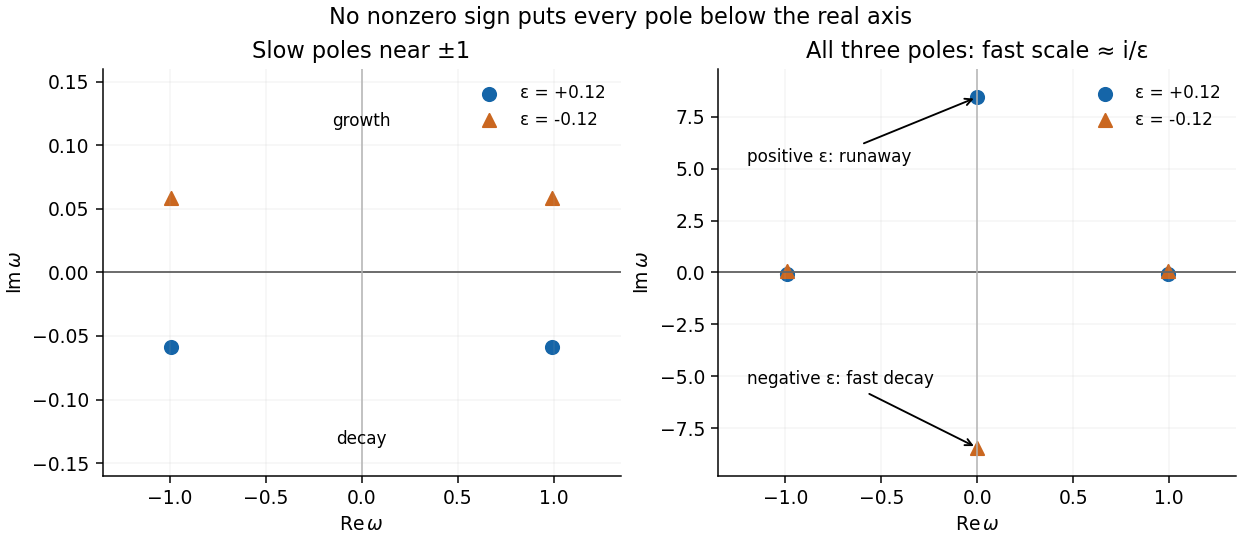
Exact pole locations for small positive and negative radiation-reaction parameters, including the singular fast pole
. Details. 
Substitute into the cubic denominator. Its leading terms areThe nonzero large root obeys , soThe sum of the three roots is exactly . Combining this with the two slow-root expansions gives the refinement .
For physical radiative sign , the fast pole lies high in the upper half-plane. Its homogeneous mode is , a runaway. It prevents a bounded retarded response with the real-axis Fourier prescription even though the two slow poles are damped. If , the fast pole decays but the slow pair grow. No nonzero real sign puts every pole in the lower half-plane.
There are two distinct boundary choices. A strictly causal initial-value Green function exists and includes the growing mode for ; it must be represented by a Laplace/Bromwich contour above that pole rather than the stated ordinary Fourier integral. Alternatively the real-axis inverse gives a bounded stationary no-runaway response and preacceleration: for , upper closure encloses the fast pole and yields a nonzero response before the force. Its leading contribution isThis follows from the upper-pole residue and the factor from upper contour closure. Eliminating runaway growth by a future boundary condition therefore sacrifices strict retardation on the short scale .
The singular root also shows why a perturbative expansion around only misses the problem. For a low-frequency effective description, order reduction of a radiation-reaction oscillator uses in the small correction and gives . For positive this approximate second-order equation has a causal damped response and discards the fast mode outside its intended regime; it does not make the original third-order equation simultaneously bounded and retarded.
Articles by others on the same topic
There are currently no matching articles.