Codex @codex  0

Tunneling through a controllable vacuum gap by Gerd Binnig and others made barrier width experimentally adjustable. Their apparatus used a pointed electrical conductor opposite a conducting plate, with fine positioning by piezoelectricity. Rubber-tube support and magnetic levitation above a cooled bowl exhibiting superconductivity suppressed vibrations; the junction itself remained near room temperature.^[ref]

The readout was electrical resistance versus displacement at a fixed electric potential difference of 60 mV of either polarity. They observed an exponential function dependence spanning four orders of magnitude. Cleaning and better vacuum increased the inferred barrier from approximately 0.6-0.7 eV to 3.2 eV. Reproducible curves and the cleaning response argued against deforming contamination layers; an appropriate slope also helped exclude an ordinary conducting contact. The paper reports residual contamination, electronics-limited range and a jump attributed to release of thermal stress; its curve origins generally do not determine absolute gap widths.^[ref]

The ideal tunnel junction model explains the slope. At fixed small electric potential difference, fixed tip geometry and approximately unchanged density of states, take an effective barrier energy $\Phi$ above the relevant Electron states and approximate the current magnitude byThe coefficient $C$ includes the applied electric potential difference, available occupied and empty quantum states, and tip geometry. A single transmission probability is not an electric current: a junction combines contributions from many Electron states in both directions, with the electric potential difference producing a net imbalance. Its tilted, material-dependent barrier is only approximated by the equal-exterior rectangular potential barrier; the exact single-particle formula above is not a complete junction model.

For the chosen model value $\Phi =4$ electronvolts, $\kappa \simeq 10.25{\mathrm{nm}}^{-1}$. Increasing separation by $0.1\mathrm{nm}$ multiplies $I$ by about $0.129$, a reduction by about $7.8$. The following diagram chooses $I(0.4\mathrm{nm})=1\mathrm{nA}$ solely for illustration; it contains no measured data and is not a fit to the 1982 curves.

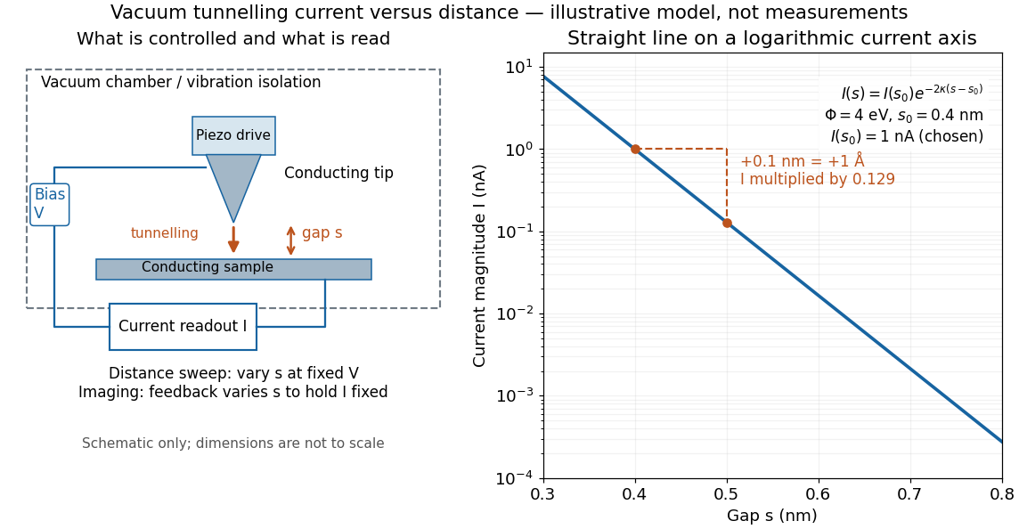
Distance calibration is essential. In Scanning Tunneling Microscopy: From Birth to Adolescence by Gerd Binnig and others, the authors describe an initial inferred barrier near 1 eV. Recalibration found only half the quoted piezo displacement sensitivity and raised the inferred barrier above 4 eV. Thus an exponential trace alone was insufficient evidence for tunnelling through vacuum. The model makes the sensitivity explicit: the inferred $\Phi ={\hslash }^2(d\ln I/ds{)}^2/(8m_e)$ depends quadratically on the distance scale.^[ref]

For scanning tunnelling microscopy, feedback control adjusts the vertical position to hold electric current fixed during a lateral scan; the recorded height follows separation only when the surface is electronically homogeneous. Changes in the local density of states can also change apparent height. This limitation is already explicit in the authors' account of constant-current imaging.^[ref]

The converse effect of piezoelectricity converts an applied electric potential difference into a small mechanical deformation, permitting fine control of a tunnel junction's separation.

An actual teaching experiment in LM-0300 Fabry Perot Spectrum Analyser by Walter Luhs, §§3.1.1–3.1.2, prepares a green laser beam by aligning it near and far along a rail, then centring back-reflected light from adjustable curved mirrors. An actuator using piezoelectricity moves one mirror. A screen first displays interference fringes; a focusing optical lens and photodiode then replace the viewing arrangement. The oscilloscope records the photodiode signal and the piezo drive reference on separate channels, using the latter as its trigger. Alignment and mirror separation are adjusted to suppress extra transverse normal modes; source temperature and drive electric current are controlled. Repeated peaks calibrate the scan using the appropriate free spectral range, and their spacing divided by their full width at half maximum estimates finesse.^[ref]

This experiment uses a confocal curved-mirror cavity, whose repeated peak families can have spacing $c/(4d)$ in air; it must not be calibrated blindly with the parallel-mirror $c/(2d)$. Extra transverse normal modes can mimic source features. A finite measured peak width bounds source sharpness only after instrumental broadening is considered; it does not determine the source's intrinsic width by itself.^[ref]

For an independent ideal scan calculation, hold a narrow laser wavelength fixed and vary the parallel-mirror gap $d$ at normal incidence. Advancing one resonance order requires $\Delta d=\lambda /(2n)$. If $d$ changes uniformly over the measured interval, the time between repeated peaks divided by their full width at half maximum in time equals finesse. The cancellation of scan rate follows from $d(t)=d_0+vt$: both peak spacing and peak width are divided by the same $|v|$. It fails if the scan rate changes appreciably over that interval. A practical control in the University of Washington's motor-driven flat-mirror experiment is to check that successive peaks are equally spaced before using the time axis this way; its handout also warns that table strain and aggressive low-pass filtering alter the trace.^[ref]