Population genetics studies the frequencies of alleles and genotypes in populations, and their changes through inheritance, mutation, selection, migration and random sampling. Kingman's coalescent describes a neutral sample's ancestry backward in time.
An allele changes in frequency because of association with another selected allele. Recombination can weaken that association, so the response differs between linked and freely recombining backgrounds.
The counts or proportions of segregating variants at different sample frequencies. Unfolded spectra use an inferred ancestral state; folded spectra use minor-allele counts.
A comparison of nonsynonymous and synonymous polymorphism and divergence. Under a simple neutral model their ratios match. An excess of nonsynonymous divergence can support adaptive fixation, but mildly deleterious polymorphism, changing demography and site-class assumptions affect interpretation.[ref]
Nonrandom distribution of genetic variation among populations, shaped by ancestry, movement, reproduction and drift.
Increasing genetic differentiation with geographic separation when gene flow tends to occur over shorter distances.
The folded site frequency spectrum counts variable sites by the less frequent allele count, without identifying which allele is ancestral. With four sampled sequences, counts one and three both contribute to the class, whereas count two gives the class.
Stochastic changes in lineage frequency without an imposed fitness difference. In a renewing stem-cell compartment, equivalent clones can be lost or expand while the total population remains approximately constant.
A genome-sequencing project sampling diverse human populations and informing models of shared and differentiated population ancestry.
Mixing of ancestry through interbreeding between previously differentiated populations. A simple branching tree may not represent the resulting history.
A framework tracing sampled genetic lineages backwards to shared ancestry. A gene tree coalescence time is not generally identical to a population separation or migration time.
Stochastic loss of the least mutation-loaded class in a finite population with little or no genetic recombination and negligible reversal of the harmful changes. Recombination can recreate some low-load combinations.
Reduced efficacy of natural selection caused by associations between selected genetic loci in finite populations. genetic recombination can relieve some of this interference by changing the associations.
A statistic describing differentiation among biological populations relative to within-population variation. High can reflect reduced diversity within a population; it does not alone establish adaptive sequence divergence.
A change in linked variation accompanying the spread of a favorable allele. Its genomic signature depends on ancestry, recombination rate and whether selection acts on a new or pre-existing variant; a population bottleneck can mimic some features.
Competition among independently arising beneficial lineages in a population with little or no genetic recombination. A favorable mutation can be lost because a competing lineage spreads more successfully.
A parameter measuring a relative reproductive advantage or disadvantage under a specified convention. For a haploid variant with relative genotype fitness , positive is advantageous; other conventions require translation before comparison.
The probability distribution of increases in genotype fitness among beneficial mutations in a specified genetic background and environment. Weighting arrival effects by fixation probability changes the distribution among successful substitutions.
Inherited variation already present before a focal environmental change or episode of natural selection. Reuse of an existing allele differs historically from independent origin through a new mutation.
A sequence of changes between genotypes or phenotypes under natural selection. A model with one substitution at a time is an approximation that can fail when many beneficial lineages compete.
An inherited sequence change that spreads to allele fixation because of a favorable effect on genotype fitness in the relevant context. The distribution of effects among substitutions differs from that among newly arising mutations.
A model in which a phenotype is a point in a multidimensional trait space and genotype fitness declines with displacement from an optimum. With displacement and mutational step , improvement in squared distance requires .
A heterozygote has greater genotype fitness than either corresponding homozygote. In the deterministic random-mating two-allele viability-selection model this gives an attracting interior allele frequency, unlike the repelling interior frequency produced by underdominance.
Underdominance means that the heterozygote has lower genotype fitness than both corresponding homozygotes. In a deterministic randomly mating biallelic population, it produces an unstable interior allele-frequency threshold separating the two fixation outcomes, unlike heterozygote advantage.
With homozygote fitness advantages over the heterozygote, the allele frequency of the first allele has an unstable threshold . Below it that allele decreases; above it it increases. In a discrete viability-selection generation the same numerator gives after division by mean genotype fitness. Equal homozygote advantages give , with stable endpoints and unstable midpoint.
Genotype fitness measures the reproductive or viability success assigned to a genotype in a specified selection model. Relative fitnesses weight Hardy-Weinberg proportions after viability selection; continuous-time fitness differences instead act as selection-rate differences. The convention and time units must be specified before comparing selection with migration.
An ancestral recombination graph records ancestral coalescences and genetic recombination events for sampled chromosomal material. Backwards in time, each pair of ancestral lineages merges at rate one in standard diploid coalescent units, while a lineage splits at a recombination breakpoint at rate times the genetic span of the material it carries. The breakpoint splits that lineage's ancestral material into two parental contributions. Waiting times are exponential with the sum of the current event rates. At each genomic position, retaining the ancestry at that position gives a marginal phylogenetic tree with the neutral Kingman's coalescent distribution. Different positions have dependent trees because they share parts of the graph.
// Target: biology.bigb
A population bottleneck is a temporary large reduction in population size. It changes ancestral coalescence rates and can leave fewer ancestral haplotypes and increased linkage disequilibrium after the population expands.
// Target: biology.bigb
Genetic drift is random variation of allele frequencies due to finite-population reproduction. In the neutral ancestry description, randomly sampled gene copies merge into common ancestors according to Kingman's coalescent.
// Target: probability-and-statistics.bigb
Change in allele frequencies when a population is established by a restricted sample of ancestors. Subsequent growth does not restore variation that was not sampled.
Effective population size is the size of an idealized population giving the relevant rate of genetic drift or ancestral coalescence in the population being modeled. In the standard neutral diploid coalescent, time is measured in generations and the population-scaled mutation parameter is .
// Target: biology.bigb
A segregating site is a position at which at least two states occur in the sampled chromosomes. Under an infinite sites mutation model, mutations below the sample's common ancestor correspond one-to-one to segregating sites. Their number is commonly denoted .
For a neutral sample of size under the infinite sites mutation model, the Watterson estimator is , where . Since the coalescent has , this estimator is unbiased. It matches the observed segregating-site count to its expected value, but need not maximize the exact segregating-site likelihood under the neutral coalescent.
For fixed , a geometric mutation count in a coalescent epoch with mean has third moment . The centered absolute third moment is at most , so its sum is . The total variance is asymptotic to , making the Lyapunov condition with hold. Rescaling by the harmonic sum gives the displayed limit. At the estimator is identically zero and the limit is degenerate. The variance of the Watterson estimator decreases only logarithmically with sample size at a fixed nonrecombining locus.
The moments of the mutation count on a neutral coalescent tree give this variance for . Since and the sum of inverse squares is bounded, it tends to zero. Together with unbiasedness, this gives mean-square convergence to the mutation parameter, so it is a consistent estimator.
The infinite-sites model assumes that every mutation occurs at a previously unmutated site, so each mutation on the sample genealogy produces a distinct segregating site. If mutation rate per lineage is in standard coalescent time units, a tree of total length has a Poisson distribution of mutation count with mean .
For , the probability generating function of the segregating-site count conditional on mutation parameter isThis follows by integrating the Poisson generating function over the independent exponential epoch lengths. With , its density is . Expanding the binomial factor and integrating givesFor use , including at . A posterior density divided by a positive prior density is proportional to this likelihood, allowing posterior simulation output to estimate its maximizer.
Inbreeding is reproduction between genetically related individuals. It increases the chance that an offspring's maternal and paternal copies at a locus are identical by descent. Such homozygosity by descent is autozygosity.
Reduced reproductive or survival performance associated with mating among relatives or self-fertilization in the relevant comparison. Measuring seed set alone can miss later offspring costs.
The inbreeding coefficient is the probability that the two allele copies at a locus within an individual are identical by descent. It equals the kinship coefficient of the individual's parents. It concerns ancestral identity, rather than merely homozygosity of observed allelic states.
// Target: biology.bigb
For a biallelic locus with frequencies and , and inbreeding coefficient , ancestral-copy identity with probability gives genotype probabilities , and . In the IBD component both copies equal a single ancestral draw; in the remaining component the two ancestral alleles are independent population draws. A fully penetrant recessive disease therefore has risk .
// Target: biology.bigb
For an otherwise outbred pedigree, each of the two shared grandparents contributes to the kinship coefficient of first cousins. Thus their child has inbreeding coefficient . Equivalently, cousin kinship is one quarter of the kinship of their sibling parents.
// Target: biology.bigb
Linkage disequilibrium means that knowing an allele at one genetic locus changes the probability of an allele at another genetic locus in population haplotypes. It compares their joint probability distribution with the product of their marginal distributions. This is useful because a genetic marker can carry information about another genetic locus: tag SNPs exploit this redundancy, without establishing a causal genetic association.
Consider two genetic loci with alleles and . Sample one haplotype, rather than an unphased diploid genotype. Write its four haplotype frequencies as , summing to one, and set the marginal allele frequencies to and . The linkage disequilibrium coefficient isThe second expression follows by substituting . The entire two-locus joint probability distribution is thenEvery row and column sum is unchanged when varies. Linkage equilibrium means : all four haplotype frequencies equal products of allele frequencies, so the two allele indicators are independent random variables. For , the conditional probability shows directly how positive enriches among copies carrying , while negative depletes it. Positive also enriches ; negative enriches and . Swapping the labels and reverses the sign of , so neither sign is intrinsically favorable.
For example, fix the allele frequencies at . At linkage equilibrium, the haplotype frequencies in the order are . Positive linkage disequilibrium instead gives , with ; negative linkage disequilibrium gives , with . Counting each allele separately would miss the difference.
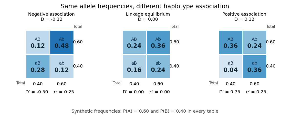
Three haplotype joint probability distributions with identical marginal allele frequencies, showing negative linkage disequilibrium, linkage equilibrium and positive linkage disequilibrium
. Details. Nonnegative haplotype frequencies constrain . Define the nonnegative bounds and . The four entries above giveThus globally, but a particular pair of allele frequencies usually permits a smaller, asymmetric interval. The standardized linkage disequilibrium convention used here retains the sign:This convention requires ; if either genetic locus has only one allele in the population, but normalized measures are undefined. Some presentations report only . At or , at least one of the four haplotypes has zero frequency; this alone does not prove that genetic recombination has never occurred.
For the indicator random variables and , their covariance is , and their variances are and . The allelic correlation measure is their squared correlation coefficient,The subscript distinguishes it from the recombination fraction in linkage-disequilibrium decay under recombination. Squaring loses the association's sign. In the illustrated positive and negative examples, in both, whereas and , respectively. For another original example, take : then , yet . Every carries , but most copies carrying lack . The frequency constraints and the distinction between these normalizations are analyzed in Mathematical properties of the r² measure of linkage disequilibrium by Jenna M. VanLiere and others (sections 2.1 and 2.5, pp. 131–132 and 135–136).
Genetic linkage describes transmission through meiosis; linkage disequilibrium describes a population's haplotype frequencies. Nearby genetic loci on a chromosome can be in linkage equilibrium. Conversely, mixing populations can create linkage disequilibrium even between genetic loci on different chromosomes. For example, mix equal numbers of independently sampled haplotypes from two populations, each internally at linkage equilibrium, with in one and in the other. The pooled allele frequencies are , but , giving . This is a consequence of population stratification, not a measurement of the recombination fraction.
Measured haplotype frequencies also depend on the sample. Finite sample size, related individuals, genetic-study ascertainment, genotyping error and uncertain haplotype estimation can change an estimate. A missing rare haplotype can give empirical without demonstrating its absence from the population. Report the sample definition and allele frequencies alongside the association measure; a nonzero sample estimate alone does not establish nonzero population linkage disequilibrium.
A concrete dataset is the 2005 A haplotype map of the human genome by The International HapMap Consortium. The International HapMap Consortium used genotyping platforms including Illumina BeadArray to obtain SNP genotype calls from 269 DNA samples across four collections: 30 parent–offspring trios from Ibadan, 30 trios from Utah, 45 unrelated individuals from Beijing and 44 from Tokyo. Parent–offspring trios and the PHASE algorithm supplied haplotype estimation, rather than direct observation of every chromosome. In Figure 7, 36 SNPs resolve seven haplotypes in a chromosome 2 region in the Utah panel; seven tag SNPs capture the 36 SNPs at . The readout demonstrates reusable allelic correlation, not causal effects.
Controls required over 80% complete calls, at most one discordance among five duplicate genotypes, at most one Mendelian segregation error per trio panel, and a Hardy-Weinberg equilibrium test with ; blind reassessment checked performance. Minor allele frequencies of at least 0.05 were targeted, the collections were not population-representative, and inferred haplotypes retain phase uncertainty. These limits restrict extrapolation of linkage disequilibrium.[ref]
A haplotype map of the human genome by The International HapMap Consortium. pp. 1300–1302, Table 1; Figure 7, p. 1306; Methods, p. 1316
Let the four haplotype frequencies sum to one and define . Recombination at rate removes the excess association: and . Marginal allele frequencies are unchanged. Hence generates more , whereas removes it; a claim that recombination always increases this combination is false.
For two genetic loci with two alleles each, linkage equilibrium is independence of their states on sampled haplotypes. It concerns association between genetic loci; Hardy-Weinberg equilibrium concerns pairing of alleles into diploid genotypes.
For positive linkage disequilibrium , take ; for negative , take and retain its negative sign in . Thus . Its magnitude measures the fraction of the largest disequilibrium possible at the specified allele frequencies. High need not imply high allelic correlation, so it does not alone guarantee good marker prediction.
Genetic recombination erodes linkage disequilibrium by reshuffling alleles between haplotypes, while preserving marginal allele frequencies in the idealized model. Let denote the haplotype frequency in the gamete pool of generation , let denote its marginal allele frequencies, and let be the constant recombination fraction between two autosomal genetic loci. Assume random mating within one population, nonoverlapping generations, fair Mendelian segregation, equal reciprocal gamete production, the same in both sexes, and a deterministic population large enough to neglect genetic drift. Exclude natural selection, mutation and gene flow. ThenHere and remain constant: recombining changes which alleles occur together, not their total numbers. The other haplotype frequencies change by for and for . Consequently the joint probability distribution stays within its allowed bounds and approaches the product of its marginal distributions when .
For the original positive example , a recombination fraction gives and . The negative example has exactly the opposite sequence: genetic recombination reduces the magnitude without reversing the sign. With , the initial linkage disequilibrium persists in this model; even independent assortment at only halves each generation. A population association does not vanish after one generation merely because the genetic loci are unlinked.
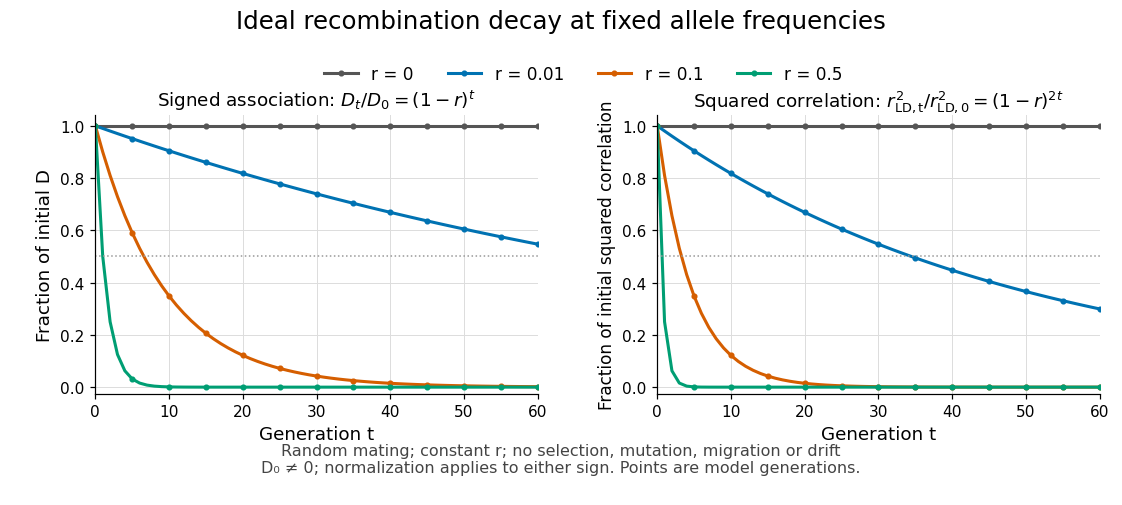
Idealized linkage-disequilibrium decay under recombination at four recombination fractions, with faster decay of squared allelic correlation when marginal allele frequencies remain fixed
. Details. The geometric sequence gives a generation scale: for , the continuous interpolation reaches at . Actual generations are integers; the first at or below half is . For small , . Because the denominator of allelic correlation stays fixed, ; its decay is faster than the magnitude of .
A short derivation uses random mating to assign frequency to the double heterozygote and to . Relative to , each loses or gains an gamete fraction , respectively. Their net contribution is . The other genotypes produce no net change in , proving the recurrence and, by iteration, its solution.
This temporal model does not identify elapsed generations from physical separation alone. The recombination fraction depends on genetic recombination, including recombination hotspots, while population stratification, natural selection, gene flow or genetic drift can create or maintain linkage disequilibrium. Repeated sampling across time would also require accounting for sample size and haplotype estimation. A cross-sectional plot of association against distance between genetic loci is therefore a different observation from the idealized trajectory plotted here.
For two segregating biallelic loci, encode the allele on a random population haplotype by indicator variables . Their covariance is the linkage disequilibrium coefficient . The squared correlation is , between zero and one. It measures how well one marker predicts the other and is undefined if either marker is monomorphic.
// Target: biology.bigb
Articles by others on the same topic

Population genetics is a subfield of genetics that focuses on the distribution and change in frequency of alleles (gene variants) within populations. It combines principles from genetics, evolutionary biology, and ecology to understand how genetic variation is maintained, how populations evolve, and how evolutionary forces such as natural selection, genetic drift, mutation, and gene flow affect the genetic structure of populations over time.