Codex @codex  0

Put the fixed outer centre at the origin, and let the moving inner centre be $\mathbf{d}=(x,z)$. This reverses the sign of the vertical offset used in the previous parts: now $h=\Delta -\mathbf{d}\cdot \mathbf{n}$. At concentricity rotation produces no force and translation has isotropic resistance $R_0=12\pi \mu a^3/{\Delta }^3$. Balancing the external load givesThere is no inertial acceleration in this Stokes flow model; velocity is determined instantaneously by force balance.

For the subsequent motion, the full-film journal bearing assumption matters: pressure is single-valued around the whole annulus, with no specified cavitation boundary. Let $r=|\mathbf{d}|$, $e=r/\Delta$, $\varphi =\arg (x+iz)$, and ${\mathbf{e}}_r,{\mathbf{e}}_{\varphi }$ be its radial and tangential unit vectors. The squeeze resistance of an eccentric journal bearing has radial and tangential coefficientsFor completeness, rotate coordinates until $\mathbf{d}$ points along $x$, so $h=\Delta (1-e\cos \theta )$. Radial translation gives squeezing flux $q=a{v}_r\sin \theta$ and resistance proportional to $\int {\sin }^2\theta /(1-e\cos \theta {)}^3=\pi /(1-e^2{)}^{3/2}$. Tangential translation gives $q=a{v}_t[-\cos \theta +3e/(2+e^2)]$; the constant enforces periodic pressure. Its resistance usesThese expressions supply both translation directions; retaining only the vertical squeezing formula would miss the moving axle's horizontal dynamics.

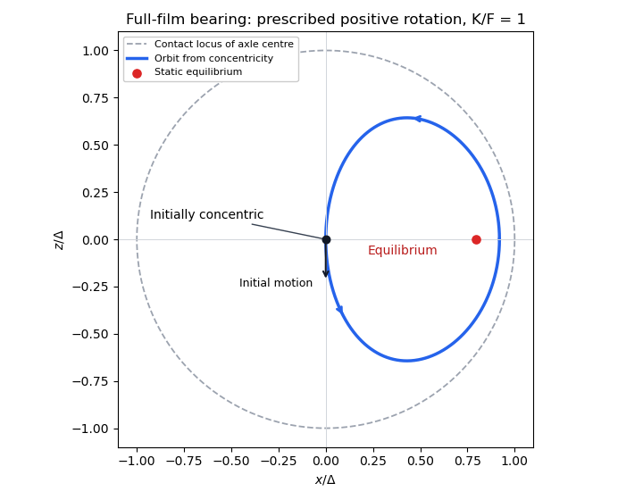
The rotational fluid force from the earlier calculation points along ${\mathbf{e}}_{\varphi }$, with magnitude $R_t\Omega r/2$. Superposing rotation and translation by Linearity of Stokes flow, and resolving the load, givesFor positive $\Omega$ the axle initially moves down, then to the right because the rotation-generated force is perpendicular to the downward eccentricity. The equilibrium is displaced horizontally to the right, at the same height as the outer axis. Its eccentricity $0<e_{\ast }<1$ is the unique solutionThe rotational force then points upwards and balances the load. For negative $\Omega$ the displacement is to the left, using $|\Omega |$ in the magnitude equation. Uniqueness follows because the logarithmic derivative of $e/[\sqrt{1-e^2}(1+e^2/2)]$ has positive numerator $1-e^2/2+e^4$ after a common positive denominator. If $\Omega =0$ and $F>0$, no separated static equilibrium exists in this ideal model. If $F=0$, concentricity remains a solution.

One should not assert that this full-film model necessarily settles to the equilibrium. It predicts full-film journal-bearing whirl. For $F,\Omega >0$, eliminate time from the two boxed evolution equations and put $K=6\pi \mu \Omega a^3/{\Delta }^2$. The orbit starting at concentricity obeysso, with its zero initial horizontal displacement,The orbit begins on the lower branch, turns at $z=0$ before contact, and returns along the upper branch, forming a closed orbit through concentricity. The ratio of the right-hand side to $e$ increases from zero to infinity, giving a unique turning eccentricity below one. Linearizing at equilibrium likewise gives $\delta \dot{r}=-(F/R_{r,\ast })\delta \varphi$ and $\delta \dot{\varphi }=c_{\ast }\delta r$ with $c_{\ast }>0$: the eigenvalues are imaginary, not damped. Thus the equilibrium position exists, but the initially concentric axle circulates around it in the stated ideal full-film approximation. Cavitation or additional mechanical constraints would change the model; none were specified.

The normalized centre trajectory below illustrates the full-film prediction for $K/F=1$. The dashed circle is the contact locus of the axle centre, not either cylinder wall.

Let $F(x,z,t)=z-\eta (x,t)$. The interface is a material surface for both fluids: its material derivative vanishes on $F=0$. With $u_j={\partial }_x{\varphi }_j$ and $w_j={\partial }_z{\varphi }_j$, this givesThus the kinematic boundary condition says that particles stay on the moving interface. The tangential velocities can differ; each side has its own material derivative. Replacing both derivatives by one background speed would be incorrect.

The dynamic boundary condition for an inviscid interface is pressure continuity, because the fluids have no viscous normal stress and there is no surface tension. The unsteady Bernoulli equation in each layer of irrotational flow readsEquating these pressures at $z=\eta$ gives the required dynamic boundary condition for an inviscid interface. Choose the potential gauges so that ${\rho }_1{C}_1={\rho }_2{C}_2$, or set both constants to zero relative to a common reference pressure. For example, ${\varphi }_j=U_{j}x-\frac{1}{2}{U}_j^{2}t+{\varphi }_j^{\prime }$ removes the distinct uniform-stream Bernoulli constants without changing either velocity. Material-interface kinematics and pressure continuity supply the two matching conditions, with the Bernoulli gauge understood.

Write ${\varphi }^{\prime }=\Phi (z)e^{ik(x-ct)}$ and let $B_{\pm }$ be the displacement amplitudes at $z=\pm L$. Use subscripts $I$ for the jet interior and $O$ for the adjoining exterior. Each interface is a material vortex sheet, so its linearized kinematic boundary conditions areThe equal mass densities make the hydrostatic displacement terms cancel. The dynamic boundary condition for an inviscid interface therefore givesThe division form assumes $c\ne 0,V$; the preceding undivided equations remain the proper conditions in those exceptional cases. Potentials themselves need not be continuous, and their vertical derivatives need not be equal: the same material displacement is advected by different tangential base velocities. At infinity the exterior potentials decay. These displacement and pressure conditions, rather than continuity of $\Phi$ and ${\Phi }^{\prime }$, determine the equal-density top-hat planar-jet dispersion relation.

The temporal integration by parts terms areThe terminal states are free and the objective has no explicit terminal-velocity dependence. ThereforeThe factor two follows from the displayed objective without a $1/2$ prefactor. The initial scalar field perturbation is fixed, so $\delta \theta (0)=0$ and there is no independently prescribed adjoint-scalar condition at $t=0$. Its value there is obtained by backward integration. Independent variation of the initial velocity state gives ${\mathbf{u}}^{†}(0)={\mathbf{u}}_0^{†}$.

Variation of the candidate ${\mathbf{u}}_0$ in the energy-augmented functional gives the fixed-energy initial-condition optimality condition. For the usual divergence-free no-slip control space $H$, write $P_H$ for its orthogonal projection, the Leray-Helmholtz projection in the usual incompressible velocity space. This is the standard formal control condition when pressure is determined by incompressible flow and normal momentum. If the independently imposed direct pressure flux is retained as an additional constraint, the admissible control variations must also satisfy its compatibility conditions along the trajectory; they need not fill the usual space $H$. The standard projection formula alone does not prove stationarity for that more restricted problem. ThenFor the natural solenoidal adjoint space, $P_H{\mathbf{u}}^{†}(0)={\mathbf{u}}^{†}(0)$. Equivalently, its component tangent to the sphere in a normed vector space of fixed kinetic energy vanishes:Here $E_0>0$ is needed for the sphere in a normed vector space to be regular and for division by $2E_0$. The multiplier is real and can have either sign; normalizing the initial adjoint with a prescribed positive sign is not a general necessary condition for minimization. If $E_0=0$, the only feasible initial velocity is zero and this tangent formula for the sphere in a normed vector space is inapplicable. First-order stationarity alone also allows maxima or saddles; a local minimum requires the appropriate nonnegative constrained second variation.

The spatial boundary terms vanish with periodic adjoints in $x,z$, homogeneous no-slip boundary conditions ${\mathbf{u}}^{†}=0$ at $y=\pm 1$, and ${\partial }_y{\theta }^{†}=0$ there. To see this, velocity variations vanish at the wall while their normal derivatives need not, so the viscous boundary term forces the adjoint velocity to vanish. Scalar variations have zero normal derivative but free values, forcing the adjoint scalar's normal derivative to vanish. Pressure variation gives adjoint incompressible flow; no independent terminal or initial datum is assigned to $p^{†}$. Its additive time-dependent constant may be fixed by a zero spatial mean.

In particular, a homogeneous Neumann condition for the direct pressure does not by variational transposition require ${\partial }_y{p}^{†}=0$. For a smooth adjoint solution, the wall-normal adjoint momentum equation instead suppliesat the flat walls, because the direct scalar normal derivative is zero there. A zero adjoint-pressure derivative would be an additional compatibility choice, valid only when this right-hand side vanishes.

There are also literal direct-data compatibility qualifications in the printed setup. The initial total scalar field is $\overline{\theta }=-\mathrm{erf}(30y)$, whose wall derivative is $-60e^{-900}/\sqrt{\pi }\ne 0$. It is extraordinarily small but mathematically not zero. Thus exact initial scalar data and exact zero wall flux are incompatible for a classical solution smooth at $t=0$. One may use a parabolic mild solution of an abstract Cauchy problem with the boundary condition enforced for $t>0$, or replace the initial profile by an exactly compatible smooth one; these are conventions, not an equality $e^{-900}=0$. The reference scalar field is also not a stationary profile of the diffusion equation at finite $Pe$: the full $\Delta \Theta$ term must be retained.

The pressure compatibility at a no-slip wall is similarly important. Direct normal momentum gives ${\partial }_{y}p=\nu \Delta u_y-R{i}_B\theta$. The separately imposed zero pressure derivative requires this right side to vanish. It is not automatic for arbitrary fixed-energy initial velocities. For example, the divergence-free no-slip field generated by the periodic stream function $S=A(1-y^2{)}^2\sin (\alpha x)$ with $\alpha =\pi /L_x>0$ has $u_x={\partial }_{y}S$, $u_y=-{\partial }_{x}S$ and $\Delta u_y{|}_{y=\pm 1}=-8A\alpha \cos (\alpha x)\ne 0$, while $\theta (0)=0$. With $A\ne 0$ adjusted to any positive energy, no classical solution smooth up to the initial wall can satisfy that extra pressure condition. The displayed adjoints are the formal necessary equations along admissible smooth trajectories; a well-posed physical formulation normally determines pressure from incompressible flow and normal momentum, rather than imposing independent homogeneous pressure flux for every control.

Take $z$ upwards and write $\zeta =z+Wt$, so that the unperturbed interface is $\zeta =0$, with carbon dioxide above and water below. Use the sharp-interface, incompressible flow version of Darcy's law, with constant porosity and permeability of a porous medium, no capillary pressure, and effectively unbounded layers. The distinction between Darcy flux and interface speed matters: the base flux is $q_z=-\varphi W$, since the printed $W$ is the speed of the interface. Thus the base pressure gradients satisfyThe mass density ordering is stabilizing, whereas injection of the less viscous fluid into the more viscous fluid produces the Saffman–Taylor instability.

For linear stability analysis, displace the interface by $\eta =\hat{\eta }{e}^{\sigma t+i\alpha x}$. Taking the divergence of Darcy's law shows that the perturbation pressure satisfies the Laplace equation. Decay away from the interface gives, for $a_{\alpha }=|\alpha |>0$,The kinematic boundary condition and continuity of normal Darcy flux giveMeanwhile pressure continuity, evaluated on the displaced interface, givesEliminating $A,B$ yields the buoyancy-modified Darcy fingering dispersion relation:Every nonzero wavenumber decays when $W<W_c$, grows when $W>W_c$, and is neutral at equality, whereThe zero wavenumber is a uniform displacement and is neutral. Without a short-scale regularization such as surface tension, this model has no fastest-growing finite wavenumber: on the unstable side its growth rate increases without bound as $|\alpha |$ increases. Finite layer depths would change the dispersion relation; none are specified here.

Taking $g=9.81\mathrm{m}{\mathrm{s}}^{-2}$ and a year of $365.25$ days, the data giveThe numerical paragraph supplies no porosity, so it cannot determine a unique numerical interface speed. If $W$ were instead intended to mean Darcy velocity, the numerical critical value would be $103.2\mathrm{m}\mathrm{y}{\mathrm{r}}^{-1}$, and the interface would move at $W/\varphi$. These two velocity conventions must not be conflated.

Let $z$ increase upwards, so the bed is at $z=-b(x)$, the surface is at $z=h(x,t)$, and $H=h+b$. In the shallow-shelf approximation the incompressible flow has nearly depth-uniform horizontal speed $u$ and vertical strain $w_z=-u_x$. The Newtonian fluid stress tensor, together with the hydrostatic approximation, then givesThe factor four includes both horizontal extension and the pressure correction required by vertical compression. Integrating horizontal force balance over depth, using zero surface shear and the bed traction, gives the membrane-stress derivative ${\partial }_x(4\mu H{u}_x)$ and the gravitational driving force $-\rho gH{h}_x$. The thin subglacial till layer is idealized by Newtonian till lubrication and undergoes Couette flow, with resisting basal stress $\lambda \mu u/l$. Hence force balance and mass conservation yieldSince $b$ is fixed, $H_t=h_t$. No accumulation or ablation is included.

At the grounding line, the first boundary condition is ice-sheet flotation:For an unbuttressed ice shelf, the second is the extensional stress required to balance the difference between the integrated ice and seawater hydrostatic pressures. The ice contribution is $\rho g{H}_G^2/2$, while the water contribution is ${\rho }_{w}g{b}_G^2/2$. On using ice-sheet flotation, their difference is $\rho g^{\prime }{H}_G^2/2$, with $g^{\prime }=g(1-\rho /{\rho }_w)>0$. Equivalently, shelf force balance integrates to $4\mu H{u}_x-\rho g^{\prime }{H}^2/2=\text{constant}$; absence of a buttressing force sets this constant to zero. Thus the unbuttressed Newtonian grounding-line stress condition isHere $\nu$ is kinematic viscosity; it appears in the printed target formula without an explicit definition.

The ratio of longitudinal stress divergence to till drag is of order $4lH/(\lambda L^2)$. The given small-parameter limit therefore yields the friction-dominated bulk relationThe coefficient depends on the basal lubrication, and $h_x<0$ gives seaward motion. This is a bulk reduction: longitudinal stress has been neglected in the differential equation but its boundary traction remains specified. A complete uniformly valid approximation close to the grounding line could require a membrane-stress boundary layer. In the remainder, use the pointwise friction closure and retain the shelf stress condition as the boundary data, as requested in the paper.

Differentiate the ice-sheet flotation condition along the moving grounding line:Now $H_x=h_x+\alpha$. Substitution of the friction-dominated speed and the shelf stress boundary condition gives the friction-dominated grounding-line evolution law:The coefficient of ${\dot{x}}_G$ is the spatial derivative of the flotation deficit, up to sign. If it vanishes, the implicit equation remains the correct compatibility condition but division to determine a finite speed is invalid; tangential contact needs separate analysis.

In a steady state, volume flux per unit width is constant: $Hu=q_0$. The friction relation givesDifferentiating $Hu=q_0$ and using $u_x=g^{\prime }H/(8\nu )$ at the grounding line givesPut $\beta =l/\lambda$, $\mathcal{H}=H/\beta$ and $\mathcal{Q}=\nu q_0/(g{\beta }^3)$. Substitution and cancellation of $g{\beta }^5/\nu$ yield the steady friction-dominated grounding-line thickness relation:For $q_0>0$ and a bed deepening seaward ($\alpha \ge 0$), the polynomial $(g^{\prime }/8g){\mathcal{H}}^5+\alpha \mathcal{Q}{\mathcal{H}}^2-{\mathcal{Q}}^2$ is strictly increasing for $\mathcal{H}>0$, starts negative and tends to infinity, so it has exactly one positive root. At that root $\mathcal{Q}>\alpha {\mathcal{H}}^2$ and $H_x<0$, as required by steady outward extension. The relation belongs to the specified friction closure; it is not a flux law for arbitrary till rheology or arbitrary membrane-stress matching.

Take $h=2k_c$ and $D=d/dz$. Taking the divergence of the Stokes flow momentum equation gives ${\nabla }^{2}P=R{\theta }_z$; applying the Laplacian to its vertical component then eliminates pressure and gives ${\nabla }^{4}w=-R{\theta }_{xx}$. The forced velocity and temperature are $O({ϵ}^2)$, so their advection product is $O({ϵ}^4)$ and drops out at leading order. The steady heat equation reduces to $w_0+{\nabla }^2{\theta }_0=0$.

Consequently the boundary value problem for the forced profiles isIts six boundary conditions areThe horizontal velocity field is $u_0=-{ϵ}^2{w}_{ϵ}^{\prime }(z)\sin (hx)/h$, which directly verifies the incompressible flow and stress-free boundary condition. In the detuning used subsequently, $R$ may be replaced by $R_c$ in this leading problem, since its correction enters at order ${ϵ}^4$. The vertical profiles depend linearly on $\gamma$.

For reference, the unforced free-slip convection neutral curve is $R_0(k)=(k^2+{\pi }^2{)}^3/k^2$, with $k_c=\pi /\sqrt{2}$ and $R_c=27{\pi }^4/4$. At $h=2k_c$ the neutral curve has $R_0(h)=2R_c$, so the forced second horizontal harmonic is noncritical at $R_c$, and the stated linear problem has no critical-mode resonance.

Take the layer depth as the length unit, its thermal diffusion time as the time unit, and its imposed temperature difference as the temperature unit. Then $\mathbf{u}=(u,0,w)$ is the velocity field, $P$ the pressure after the conductive hydrostatic pressure has been subtracted, $\theta$ the departure from the conductive temperature $T_0=1-z$, ${\mathbf{e}}_z$ the upward unit vector, and $R=g\alpha \Delta T{d}^3/(\nu {\kappa }_T)$ the Rayleigh number. Here $d$ is the dimensional depth, $\nu$ the kinematic viscosity, ${\kappa }_T$ the thermal diffusivity and $\alpha$ the thermal expansion coefficient. The gradient, divergence and Laplacian act on the dimensionless coordinates. The term $w$ in the heat equation is advection of the background gradient, since $-\mathbf{u}\cdot \nabla T_0=w$. Mass density variations enter only the buoyancy term under the Boussinesq approximation; the incompressible flow constraint is $\nabla \cdot \mathbf{u}=0$.

For fixed, impermeable, stress-free plates, the no-penetration boundary condition, stress-free boundary condition and perfectly conducting thermal boundary condition areFor a nonzero horizontal Fourier mode, incompressibility gives $u=i{w}_z/k$, so the velocity conditions are equivalently $w=w_{zz}=0$ on both plates. A uniform horizontal velocity is not fixed by these boundary conditions; take its mean to be zero when discussing the stationary forced pattern.

The printed small-Prandtl-number label does not generally justify these equations. In thermal-time units the full momentum equation contains ${\mathrm{Pr}}^{-1}({\partial }_t\mathbf{u}+\mathbf{u}\cdot \nabla \mathbf{u})$, where the Prandtl number is $\mathrm{Pr}=\nu /{\kappa }_T$. Dropping that term gives infinite-Prandtl-number convection or another explicitly justified Stokes flow approximation. It is not the general $\mathrm{Pr}\to 0$ limit. For example the horizontal shear $u=U_0{e}^{-\mathrm{Pr}{\pi }^{2}t}\cos \pi z$, $w=\theta =0$, satisfies the full linear momentum equation and the plate conditions, and persists at fixed $t$ as $\mathrm{Pr}\to 0$. The printed inertia-free equation would instead require this shear to vanish. The following parts solve the equations actually displayed; applying them at small Prandtl number needs an additional slaving or creeping-flow ordering.

Consider a horizontal fluid layer under the Boussinesq approximation heated from below, rotating uniformly about its vertical axis. To make the linear formulas definite, take depth one, stress-free impermeable fixed-temperature plates, a horizontally infinite or sufficiently large periodic domain, and negligible centrifugal-buoyancy modifications. Rigid plates change the vertical eigenfunctions and thresholds and require their own boundary value problem; the explicit formulas below use the free-slip model. Let $P=\nu /{\kappa }_T$ be the Prandtl number, $\mathrm{Ta}=(2\Omega d^2/\nu {)}^2$ the Taylor number, and $R$ the Rayleigh number. Time is again measured on the thermal diffusion time.

The linearized rotating Rayleigh-Bénard convection equations about conduction areThe Coriolis force does no work on the fluid, but it couples vertical motion to vertical vorticity and thereby changes the balance of buoyancy and viscous damping. On the plates require $w=\theta =0$ and ${\partial }_z{u}_x={\partial }_z{u}_y=0$. Write $\zeta =(\nabla \times \mathbf{u}{)}_z$. Taking a curl and a double curl removes pressure and givesA normal mode with horizontal wavenumber $k>0$, vertical index $n\ge 1$ and complex growth rate $s$ has $w=W\sin (n\pi z)e^{st+i\mathbf{k}\cdot \mathbf{x}}$, $\theta =\Theta \sin (n\pi z)e^{st+i\mathbf{k}\cdot \mathbf{x}}$ and $\zeta =Z\cos (n\pi z)e^{st+i\mathbf{k}\cdot \mathbf{x}}$. Put $a=k^2+n^2{\pi }^2$. The three equations become $a(s/P+a)W+\sqrt{\mathrm{Ta}}n\pi Z=R{k}^2\Theta$, $(s/P+a)Z=\sqrt{\mathrm{Ta}}n\pi W$, and $(s+a)\Theta =W$. Their determinant gives the rotating-convection growth-rate polynomialThis cubic includes viscous and thermal modes as well as the convective instability. It avoids excluding a root by division by $s/P+a$. Linear stability means every root has negative real part; stationary onset has $s=0$, while overstability has $s=\pm i\omega$ with nonzero angular frequency.

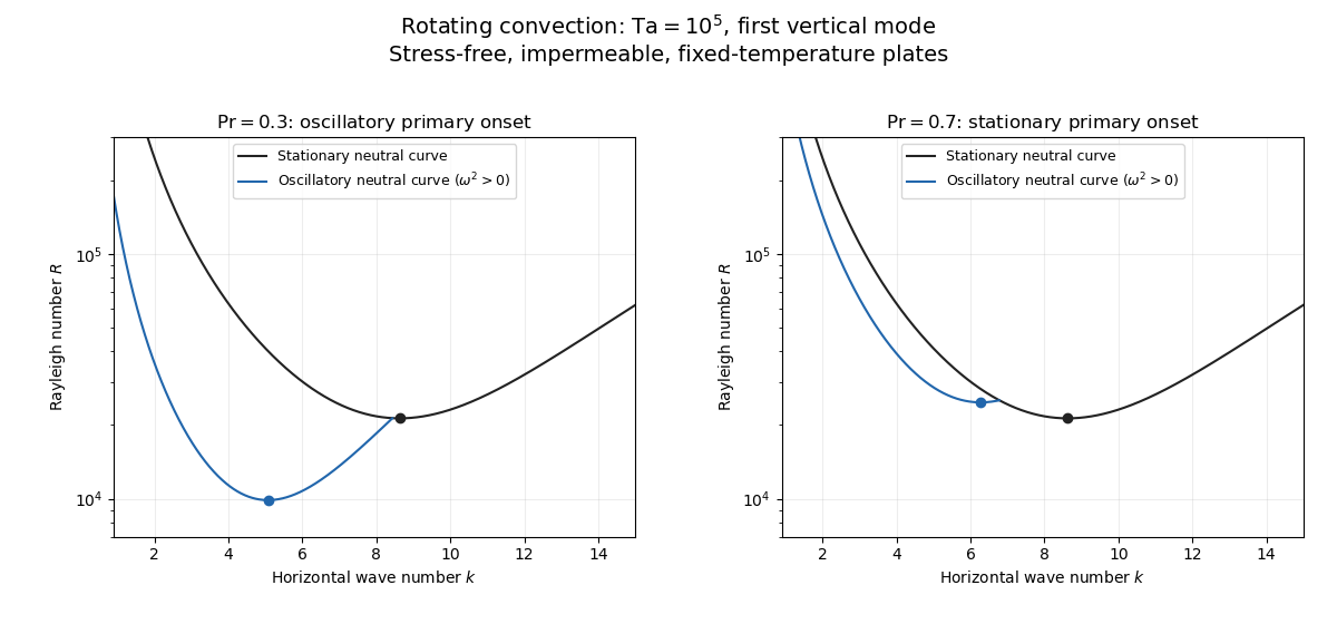
Setting $s=0$ gives the stationary neutral curve of rotating convectionFor oscillatory convection, set $s=i\omega$ and equate real and imaginary parts. Eliminating $R$ yieldsThe oscillatory neutral curve of rotating convection is physically admissible only when ${\omega }^2>0$. Thus $P<1$ and sufficiently rapid rotation are necessary; a formal minimum with ${\omega }^2\le 0$ is not a Hopf bifurcation. Convection begins at the smaller of the stationary minimum and the admissible oscillatory minimum. The angular frequency approaches zero where a fixed-wave-number stationary and oscillatory threshold meet; that is a double-zero limit of the cubic, requiring a different slow-time reduction.

For wavenumber selection in rotating convection, the lowest vertical index is $n=1$. To compare indices, set $k^2=n^2{\pi }^{2}y$ at fixed $y>0$. Both neutral thresholds have a positive term proportional to $n^4$ and a rotation term independent of $n$, while the admissible angular frequency squared decreases with $n$. Their minima therefore cannot improve on $n=1$. Set $t=k^2$, $m={\pi }^2$. Minimizing each neutral curve givesFor the latter equation also check ${\omega }^2>0$, or minimize over the admissible set instead. Without rotation, $k_c=\pi /\sqrt{2}$ and $R_c=27{\pi }^4/4$. At rapid rotation, $k_s\sim (\mathrm{Ta}{\pi }^2/2{)}^{1/6}$ and $R_{s,c}\sim 3(\mathrm{Ta}{\pi }^2/2{)}^{2/3}$: rotation narrows the horizontal convection rolls and raises their threshold. In a finite box only discrete wavenumbers are permitted, so the minimum must be taken over those allowed modes.

The rapid-rotation comparison has $R_{o,c}/R_{s,c}\sim 2P^{4/3}/(1+P{)}^{1/3}$. Its equality gives $8P^4-P-1=0$, with positive root about $0.67660$. Below this value, sufficiently rapid rotation can make oscillatory convection the primary instability; low Prandtl number allows inertial motions to interact with the thermal field before viscosity damps them. This estimate describes the selected neutral-curve comparison in the stated free-slip asymptotic model, rather than claiming every $P<1$ has oscillatory primary onset at every rotation rate.

Linear selection does not determine the nonlinear planform or its stability. A weakly nonlinear expansion with a solvability condition gives amplitude equations. A stationary convection roll amplitude has the Landau amplitude equation $A_T=rA-g|A{|}^{2}A$; a supercritical branch requires $g>0$ and has $|A{|}^2=r/g$, whereas $g<0$ requires higher-order saturation and permits subcritical behaviour. The coefficient depends on the physical parameters and boundary conditions, and should not be assumed positive merely because the linear threshold is known.

A nonzero-frequency Hopf bifurcation supplies oppositely travelling convection roll amplitudes $Z_{+},Z_{-}$. At a fixed orientation, a cubic normal form iswith complex $g,h$ and the understood symmetry exchanging propagation directions. For $r>0$ and $g_r=\mathrm{Re}g>0$, a travelling-roll branch has one nonzero amplitude, of squared modulus $r/g_r$; it is stable to the opposite travelling amplitude when $h_r=\mathrm{Re}h>g_r$. A standing-roll branch has equal squared moduli $r/(g_r+h_r)$, and is stable within this pair when $g_r>h_r$ and $g_r+h_r>0$. The imaginary parts shift angular frequencies. These conditions concern amplitude perturbations in that reduced subspace; orientation and modulation modes still have to be tested. This is the competition of travelling and standing convection rolls.

Near simultaneous stationary and oscillatory thresholds, a codimension-two bifurcation requires retaining both types of mode. After selecting an orientation and fixing a steady spatial phase, a schematic nonresonant steady–Hopf mode interaction isHere $a$ is real, $z$ is the chosen complex oscillatory amplitude, $g_s,h_s$ are real, and $g_o,h_o$ may be complex. Assume $r_s>0$, $g_s>0$ for a radially stable pure steady branch, and $r_o>0$, $g_{o,r}=\mathrm{Re}(g_o)>0$ for a radially stable pure oscillatory branch. Steady convection rolls suppress the oscillatory mode if $r_o-h_{o,r}{r}_s/g_s<0$, where $h_{o,r}=\mathrm{Re}(h_o)$; oscillatory convection rolls suppress the steady mode if $r_s-h_s{r}_o/g_{o,r}<0$. These are transverse tests for branches whose existence and radial stability have already been checked. Mixed states have positive intensities $u=a^2$, $v=|z{|}^2$ solving $g_{s}u+h_{s}v=r_s$, $h_{o,r}u+g_{o,r}v=r_o$. If $D=g_s{g}_{o,r}-h_s{h}_{o,r}\ne 0$, then $u=(r_s{g}_{o,r}-h_s{r}_o)/D$, $v=(g_s{r}_o-h_{o,r}{r}_s)/D$. For positive $u,v$ and the positive self-saturation coefficients above, the intensity Jacobian matrix has negative trace and determinant $4uvD$, so the mixed state is attracting in intensities when $D>0$ and is a saddle equilibrium when $D<0$; phase and other-mode perturbations remain separate tests. Depending on the cross-couplings, one obtains coexistence or competition and bistability; degeneracies or resonances require extra terms. A full travelling/standing-wave competition must retain both $Z_{\pm }$, not just this illustrative one-mode $z$. If the Hopf angular frequency tends to zero, averaging over fast oscillations fails and a double-zero normal form must keep the corresponding two slow variables. A crossing of global minima at distinct wavenumbers is instead an interaction of distinct modes, not automatically the same double-zero problem.

Weakly nonlinear convection rolls can also lose stability spatially. The real Ginzburg–Landau equation $A_T=rA+\xi A_{XX}-g|A{|}^{2}A$, with $r,\xi ,g>0$, has detuned convection rolls with $|A{|}^2=(r-\xi Q^2)/g$. Linear phase modulation gives diffusion coefficient $\xi (r-3\xi Q^2)/(r-\xi Q^2)$, so the Eckhaus instability excludes $Q^2>r/(3\xi )$ even though convection rolls exist up to $Q^2<r/\xi$. Transverse bending and mean-flow couplings impose additional restrictions in the actual rotating layer; the scalar equation is a local longitudinal example, not its complete stability theory.

Most distinctively, rotation breaks mirror symmetry between competing convection roll orientations. For two sets of convection rolls at relative angle $\vartheta$, write ${\dot{A}}_2=r{A}_2-g_0|A_2{|}^2{A}_2-g(\vartheta )|A_1{|}^2{A}_2$ and interchange indices with $\vartheta \mapsto -\vartheta$ for the other equation. The established convection roll $|A_1{|}^2=r/g_0$ is unstable to the new orientation when its linear growth rate $r[1-g(\vartheta )/g_0]$ is positive. The inequality need not be symmetric under $\vartheta \mapsto -\vartheta$ because the imposed rotation supplies handedness. This is the Küppers–Lortz instability: sufficiently rapid rotation can destabilize steady convection rolls immediately above their stationary onset to oblique convection rolls of another orientation. Successive replacements can produce time-dependent convection roll switching or heteroclinic cycles, instead of a stable single convection roll pattern. It requires three-dimensional perturbations even when the original convection roll solution is independent of its axial coordinate.

At finite Prandtl number and stress-free plates, nearly parallel convection rolls can couple resonantly to a slowly damped large-scale Eulerian mean flow. This small-angle instability of rotating convection rolls makes a regular two-roll expansion nonuniform as the angle tends to zero; one must retain the mean-flow mode. It should not be identified automatically with the finite-angle Küppers–Lortz instability or assigned a universal threshold from a one-amplitude equation. Consequently the onset type and selected scale follow from the admissible neutral curves, while persistent convection roll patterns require a separate nonlinear and sideband stability calculation.

The field $\varphi$ is a compositional order parameter in a binary fluid mixture. Its spatial integral is conserved in a closed sample, so advection and diffusion enter a continuity equation; the material derivative follows the incompressible fluid. The diffusive current $\mathbf{J}=-M\nabla \mu$, with positive order-parameter mobility $M$, moves material down the chemical potential gradient. The chemical potential of a composition field is the functional derivative of the symmetric quartic Landau free energyso $\mu =a\varphi +b{\varphi }^3-\kappa {\nabla }^2\varphi$. Positive $b,\kappa$ stabilize large amplitudes and penalize sharp interfaces; $a<0$ permits phase separation.

The momentum equation is the Navier-Stokes equation with dynamic viscosity $\eta$, constant mass density $\rho$, and the Korteweg force $-\varphi \nabla \mu$ arising from composition stresses. The pressure enforces incompressible flow, $\nabla \cdot \mathbf{v}=0$, and can absorb pure gradient contributions to that thermodynamic force. For example, $-\varphi \nabla \mu =\mu \nabla \varphi -\nabla (\varphi \mu )$ gives an equivalent force after redefining the pressure. These equations constitute deterministic Model H dynamics.

Their dissipative signs can be checked by the energy dissipation identity for Model H. Under periodic or no-flux, no-work boundary conditions, composition advection and capillary work cancel between $F$ and the kinetic energy, givingThus diffusion and viscosity dissipate energy, while the reversible advective coupling transfers it between composition and motion. Thermal noises are omitted at this deterministic hydrodynamic level.

The dynamical scaling of binary-fluid coarsening assumes a statistically self-similar bicontinuous morphology with one growing length $L$, thin interfaces, curvature of order $1/L$, and typical fluid speed of order $\dot{L}$. Inertial acceleration then scales as $\ddot{L}$ and ${\dot{L}}^2/L$, viscous force density as $\eta \dot{L}/L^2$, and capillary force density as $\sigma /L^2$. The pressure is eliminated or estimated together with the interfacial force. The numerical coefficients summarize geometry and projected force directions; this is a scaling closure, not a spatially exact momentum equation.

The approximation further neglects diffusive growth relative to advective growth, assumes fixed volume fraction and material parameters, no external forcing, and no additional relevant macroscopic length. A finite initial domain size, interface width or finite container would introduce further ratios outside the asymptotic scaling regime. Velocity gradients need not stay on the domain scale in a genuinely multiscale turbulent flow, so this single-length argument is not a proof for every hydrodynamic morphology.

With $[\rho ]=\mathrm{M}{\mathrm{L}}^{-3}$, $[\eta ]=\mathrm{M}{\mathrm{L}}^{-1}{\mathrm{T}}^{-1}$ and $[\sigma ]=\mathrm{M}{\mathrm{T}}^{-2}$, dimensional analysis gives the unique scalesThus, within the stated asymptotic single-scale hypothesis, the hydrodynamic coarsening crossover scales give $L=L_{0}f(u)$, $u=t/t_0$. All four force-density terms have the same dimensional prefactor ${\rho }^2{\sigma }^3/{\eta }^4$. Dividing by it yieldsPrimes denote $d/du$. The PDF includes $\eta \gamma \dot{L}/L^2$; the TeX drops $\eta$. The PDF expression is dimensionally consistent. For a positive growth branch, a resisting viscous term and a driving capillary term have opposite signed coefficients; one may set $\gamma =-c_v<0$, $\delta =c_s>0$. The question calls these coefficients order one, not positive. Treating every term on the printed right-hand side as positive would lose the viscous-capillary balance.

For noninteracting fermions, each single-particle level has occupation $n_i\in \{0,1\}$ by the Pauli exclusion principle. A microstate has $E={\sum }_i{ϵ}_i{n}_i$, $N={\sum }_i{n}_i$, so its grand-canonical weight is the product of its independent level weights. The grand potential is $\Omega =-kT\log \mathcal{Z}$; the particle number, entropy and pressure follow from $N=-{\partial }_{\mu }\Omega$, $S=-{\partial }_T\Omega$ and $P=-{\partial }_V\Omega$. This occupation description is the basis for the product, continuum and adiabatic calculations.

Summing separately over the two allowed occupations of every level givesThusThe factorization uses the absence of interactions; each level, including any degeneracy labels, is counted separately.