Codex @codex  0

For an ideal projective measurement with the Lüders rule, condition on both an initial quantum state preparation and a final successful postselection. Its outcome probabilities are proportional to $|⟨b|P_j|a⟩{|}^2$, where $a$ is the forward-evolved initial state and $b$ the backward-evolved final state. The normalization must be nonzero. The expression is symmetric in these two boundary states, although its derivation uses the ordinary Born rule and conditional state update.

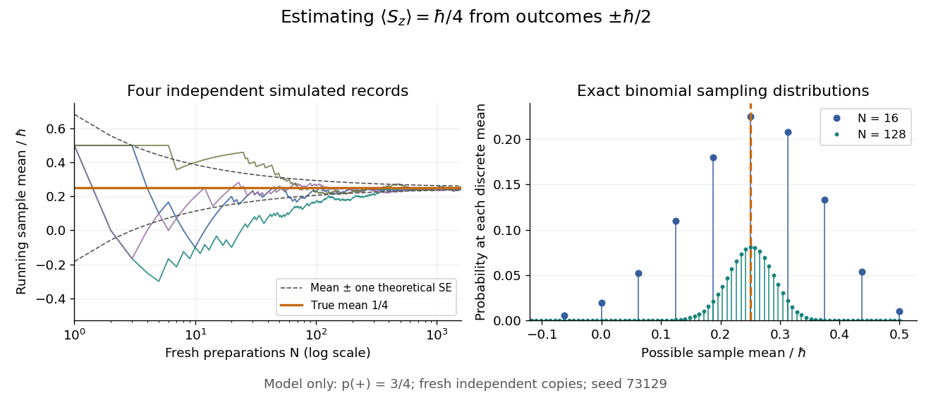
Prepare a fresh copy of the same quantum state for each trial and measure the same observable. If preparations and readouts are independent, the outcomes $X_i$ are independent and identically distributed random variables with the Born rule probability distribution. Their sample mean is an unbiased estimator of the expectation value:The law of large numbers explains convergence of the sample mean, while the standard error describes its finite-sample spread. It takes four times as many independent trials to halve that standard error. This reduces estimation error; it does not reduce the quantum uncertainty of a single prepared copy.

For the spin expectation value, let $n_{+}$ and $n_{-}$ be the two outcome counts, with $N=n_{+}+n_{-}$. ThenThe binomial distribution gives the exact sampling model. For $\theta =\pi /3$, the standard error is $\hslash \sqrt{3}/(4\sqrt{N})$: approximately $0.1083\hslash$ for $N=16$ and $0.03827\hslash$ for $N=128$. A run can fluctuate away from the predicted mean even as its typical spread decreases.

Repeatedly measuring one surviving system is a different protocol. Under the ideal Lüders rule, outcome $a_r$ leaves $P_r|\psi ⟩/\sqrt{p_r}$ when $p_r>0$. With no intervening change of observable or dynamics moving the state out of that eigenspace, the next projective measurement returns $a_r$ with certainty. Such a record is correlated and does not sample the original Born rule distribution independently. The quantum nondemolition measurement discussion describes this repeatability; fresh quantum state preparations supply the ensemble needed for the estimator above.

The expectation value of a quantum observable is the expected value of its measurement outcome random variable in a specified quantum state. It predicts the mean of outcomes from many identical quantum state preparations. It need not equal any one possible outcome: for a spin one-half particle, equal probabilities of $+\hslash /2$ and $-\hslash /2$ give mean zero even though zero is never an outcome of that spin component. Here $\hslash$ is the reduced Planck constant.

Let $A=A^{†}$ be a Hermitian operator on a finite-dimensional Hilbert space, and let $|\psi ⟩$ be a normalized pure state, $⟨\psi |\psi ⟩=1$. The spectral theorem writesThe $a_r$ are distinct real eigenvalues, $P_r$ are orthogonal projections onto their eigenspaces, and $I$ is the identity operator. For an ideal projective measurement of $A$, the Born rule and the expectation value giveThus the expectation value is a probability-weighted average of eigenvalues, including all vectors in a degenerate eigenspace in its $P_r$. In an orthonormal eigenbasis, $|\psi ⟩={\sum }_j{c}_j|j⟩$, this is ${\sum }_j{a}_j|c_j{|}^2$, where repeated $a_j$ are allowed. The weighted average lies between the smallest and largest eigenvalues; it can lie in a gap between them. The statistical meaning and operator expression are connected in this way in the authored treatment of average energies.^[ref]

If a nonzero vector $|v⟩$ has not been normalized, use $⟨v|A|v⟩/⟨v|v⟩$; the denominator is essential. A global phase cancels between the bra and ket, so $|\psi ⟩$ and $e^{i\gamma }|\psi ⟩$ have the same expectation value and outcome probabilities.

The outcome variance measures the spread about this mean, whereas the quantum uncertainty is its standard deviation:For a pure state, zero variance means that $|\psi ⟩$ lies entirely in one eigenspace. That eigenspace need not be one-dimensional. Knowing only a mean generally does not determine the entire outcome probability distribution.

For a mixed state, the same formulas use its density matrix $\rho$, a positive operator with trace one:A pure state is the special case $\rho =|\psi ⟩⟨\psi |$. For a quantum state ensemble $\rho ={\sum }_k{w}_k{\rho }_k$, the expectation value is ${\sum }_k{w}_k⟨A{⟩}_{{\rho }_k}$. This linearity is useful when preparations vary between trials; different quantum state ensembles can have the same density matrix.

These formulas require no operator-domain qualifications in finite dimension. For an unbounded self-adjoint operator, the spectral theorem instead gives a spectral probability measure; a finite mean requires an integrable absolute first moment, and finite variance requires a finite second moment. Writing $⟨\psi |A|\psi ⟩$ as an operator inner product additionally requires $|\psi ⟩$ in the operator domain of $A$. The quadratic form of a positive quantum Hamiltonian explains the useful wider form-domain version.

An ontological model associates each quantum state preparation with a probability distribution over underlying physical states $\lambda$. A measurement in quantum mechanics's response probabilities depend on its specification and $\lambda$, sum to one, and reproduce the Born rule when averaged over the preparation distribution. The model need not assign deterministic outcomes. Overlap or disjointness of preparation measures defines the psi-epistemic model versus psi-ontic model distinction.

The useful object is the Choi state of the entanglement-breaking channel. Put $d_A=\dim {\mathcal{H}}_A$, introduce a reference $R$ with the same computational basis as $A$, and use the normalized maximally entangled stateThe entanglement-breaking channel makes $C_{RB}$ a separable quantum state. Its partial trace is ${\mathrm{Tr}}_B{C}_{RB}=I_R/d_A$, because $\mathcal{E}$ is a quantum channel. Write a separable positive operator decompositionDiscard any term with $\mathrm{Tr}{\beta }_y=0$: a positive operator with zero trace is zero. DefineEach ${\tau }_y$ is a density operator. Each $E_y$ is a positive operator, and taking the matrix transpose of the partial trace identity givesThus the $E_y$ form a POVM. In this reference-first convention, the Choi reconstruction formula isThe factor $d_A$ is essential because we used a normalized Choi state. A measurement channel storing the outcome $y$, followed by the prescribed quantum state preparation of ${\tau }_y$, has precisely this action on every linear operator $L$. The desired factorization is therefore

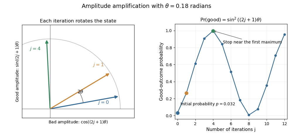
Let $\Pi$ be the orthogonal projection onto the good linear subspace $\mathcal{G}$, and let $|\psi ⟩$ be a prepared unit vector with $p=⟨\psi |\Pi |\psi ⟩$. For $0<p<1$, defineThe amplitude amplification theorem states that, if the reflection operators about the initial state and the good subspace can be implemented, the iterationsatisfiesTo prove it, the two reflections preserve the linear span of $|g⟩,|b⟩$. In this ordered orthonormal basis, direct multiplication givesMultiplying this rotation matrix by $(\sin \alpha ,\cos \alpha {)}^T$ replaces $\alpha$ by $\alpha +2\theta$, proving the formula by mathematical induction.

For known $0<p\le 1/2$, choose $j$ to be a nearest nonnegative integer to $\pi /(4\theta )-1/2$. Then $|(2j+1)\theta -\pi /2|\le \theta$, so measurement finds the good subspace with probability at least $1-p$, using $O(p^{-1/2})$ iterations. For $p>1/2$, measurement of the initial state already has constant success probability. If $p=1$ success is certain; if $p=0$ these reflections cannot create any good component. If $|\psi ⟩=A|0⟩$, the initial-state reflection is $A(2|0⟩⟨0|-I)A^{†}$, implemented using quantum state preparation and its inverse quantum circuit.

The usual sufficient input promises for the HHL algorithm are efficient quantum state preparation of the nonzero vector $b$, efficient access to a sparse matrix $A$ with at most $\mathrm{poly}(n)$ nonzero entries per row, and a condition number $\kappa ={\lambda }_{\max }/{\lambda }_{\min }=\mathrm{poly}(n)$ after an efficiently known normalization. Both the positions and values of the nonzero matrix elements must be computable coherently in polynomial time. More generally, efficient Hamiltonian simulation can replace the sparsity promise. We assume $A$ is invertible; if zero eigenvalues occur, one must instead restrict $b$ to their orthogonal complement and specify the desired inverse on that support.

With $a={\lambda }_{\max }$ and a known bound $\kappa$, choose $c=a/\kappa \le {\lambda }_{\min }$. The HHL controlled reciprocal rotation then succeeds with probabilityThis is the required inverse-polynomial lower bound. In the usual approximate algorithm, inverse-polynomial requested error also gives polynomial runtime under these input promises. The original HHL paper states the dependence on sparsity, conditioning, and accuracy.

There is a qualification for a literally exact version. Representability of the eigenvalues in $n$ bits does not itself make exact quantum phase estimation efficient: using $e^{2\pi iA}$ requires controlled powers corresponding to evolution times as large as $2\pi 2^{n-1}$. Under the paper's idealization we may describe their exact action, but polynomial runtime for that exact circuit additionally requires efficient implementations of those controlled powers, or equivalent efficient exact spectral access. Assuming an operation executes exactly does not bound its cost. This distinction is recorded in cost of exact phase estimation on a dyadic spectrum.

The essential requirement is an efficient quantum state preparation circuit $B$ satisfyingA standard sufficient promise is that $b$ has only $\mathrm{poly}(\log N)$ nonzero components, with their positions and values classically computable to the required precision in $\mathrm{poly}(\log N)$ time, and with efficiently computable normalization. More structured dense vectors are also allowed whenever cumulative weights or an equivalent data-access oracle permit amplitude encoding in polylogarithmic time. Without such a promise, merely loading $N$ arbitrary classical entries already costs $\Omega (N)$ and removes the claimed exponential dependence on dimension.

Independently operated quantum state preparations are assumed to produce independent underlying physical states. Their joint preparation measure factors into the single-system measures. This ontic factorization is an additional assumption, not a consequence of operational independence alone. It turns a common single-system overlap of mass $\epsilon$ into a common $n$-system overlap of mass ${\epsilon }^n$ in the PBR theorem.

Preparation uncertainty describes the outcome spread intrinsic to a specified quantum state preparation. Operationally, prepare many copies of the same quantum state, measure position on one group and momentum on another, and estimate the two variances. Ideal measurements still have the spreads predicted by the Born rule. No earlier position measurement need occur in the momentum group. The Heisenberg uncertainty relation constrains these two distributions belonging to the same preparation.

Measurement backaction concerns how a particular measurement in quantum mechanics changes a quantum state. Instrument resolution concerns how its reported outcomes relate to the intended observable. Those questions require a model of the instrument and its interaction with the system. Substituting an instrument error and an induced change for $\Delta x$ and $\Delta p$ in the Heisenberg uncertainty relation does not follow from its proof. The practical value of preparation uncertainty is that it bounds achievable input spreads before any such instrument model is chosen.

A measurement in quantum mechanics turns a quantum state preparation into a classical outcome, such as a detector label. Two questions must be distinguished: how likely is each outcome, and what quantum state remains conditional on that outcome? A positive operator-valued measure answers the first; a quantum instrument answers both. This distinction is useful whenever a measured system participates in a later experiment, including quantum state tomography and measurement-based quantum feedback.

For a density operator $\rho$, the Born rule gives $p_m=\mathrm{Tr}(E_m\rho )$, where the $E_m$ are positive operators satisfying ${\sum }_m{E}_m=I$. Here $I$ is the identity operator, and $\mathrm{Tr}$ denotes the trace. Positivity makes every $p_m$ nonnegative; completeness makes their sum one. For a pure state, $\rho =|\psi ⟩⟨\psi |$ and $p_m=⟨\psi |E_m|\psi ⟩$. A projective measurement is the special case in which the $E_m$ are orthogonal projections onto mutually orthogonal subspaces.

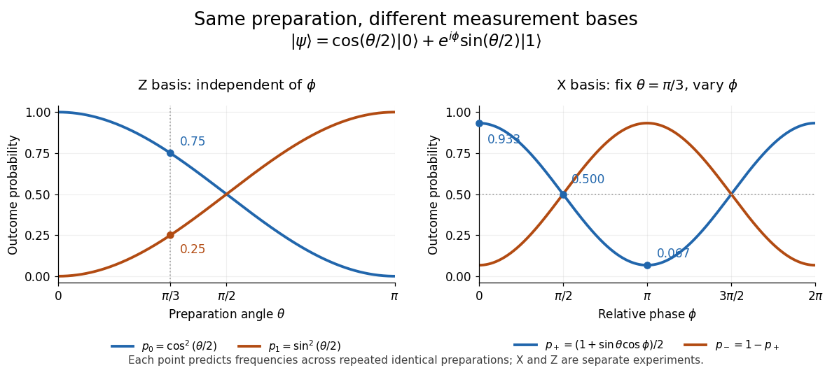
For a qubit, choose the computational basis and write a normalized pure state, up to global phase, asThe angle $\varphi$ is a relative quantum phase; at the poles it does not distinguish states. Measuring the Pauli matrix $Z$ reports $+1$ for label zero and $-1$ for label one, withThese probabilities describe repeated identical preparations. They do not assign a hidden, pre-existing value to every possible measurement basis.

The Born rule grew out of Max Born's 1926 work on quantum scattering: squared probability amplitudes determine the relative frequencies of scattering outcomes. Born explained this statistical interpretation again in his 1954 Nobel lecture. This probability law does not by itself select a post-measurement state. ^[ref]; ^[ref].