Codex @codex  0

Use a dimensionless statistical Hamiltonian $\mathcal{H}=H/(k_{B}T)$, so that the partition function is $Z={\sum }_s{e}^{-\mathcal{H}(s)}$. Choose a normalized blocking kernel $B(S\mid s)$ with ${\sum }_{S}B(S\mid s)=1$. For the majority example it is one when every block has its prescribed majority, and zero otherwise. Define the coarse statistical Hamiltonian by the displayed sum. Then an elementary interchange of finite sums provesThe probability of a retained pattern is therefore its original marginal probability. For any observable $A(S)$ of the retained variables,This is the sense in which elimination preserves predictions for retained information. It does not reconstruct every microscopic observable from a block sign.

Next express positions in units of the enlarged spacing: $x^{\prime }=x/b$, where $b>1$. In a continuum version, rescale the retained scalar field as well to restore a chosen gradient energy coefficient; any change in the integration measure contributes to the field-independent term. The result is a new set of dimensionless couplings. Repeating the procedure defines a renormalization-group flow. Additional interactions and the additive constant generally appear, even if the starting statistical Hamiltonian was simple. Keeping only a few terms is an approximation; the equality of partition functions above applies to the complete coarse weight. See also the Wilsonian coarse-grained statistical Hamiltonian for integration over fast Fourier modes.

For a Hermitian scalar field in a positive-norm Hilbert space with a Lorentz-invariant vacuum, the spectrum condition and completeness give the connected vacuum two-point function as a superposition of free mass-shell functions. Define the Källén–Lehmann spectral density by $\tilde{W}(p)=2\pi \theta (p^0)\rho (p^2)$, where $W(x)=⟨0|\varphi (x)\varphi (0)|0⟩$ and its vacuum expectation value has been subtracted if nonzero. Squared intermediate-state matrix elements make $\rho$ a nonnegative measure supported on nonnegative mass squared. Applying time ordering to each free mass shell gives the displayed Feynman propagator representation, using $i\Delta =⟨T\varphi \varphi ⟩$ and signature $(+---)$. Its positivity does not automatically extend to gauge-variant fields in an indefinite auxiliary space.

The Laplacian takes the divergence of a scalar field's gradient. For a real-valued function $f$ on an open region of Euclidean space, with continuous partial derivatives through order two, its expression in a Cartesian coordinate system isThus the Laplacian, also called the Laplace operator, adds the coordinate second derivatives; equivalently it is the matrix trace of the Hessian matrix. Its output is another scalar field.^[ref]

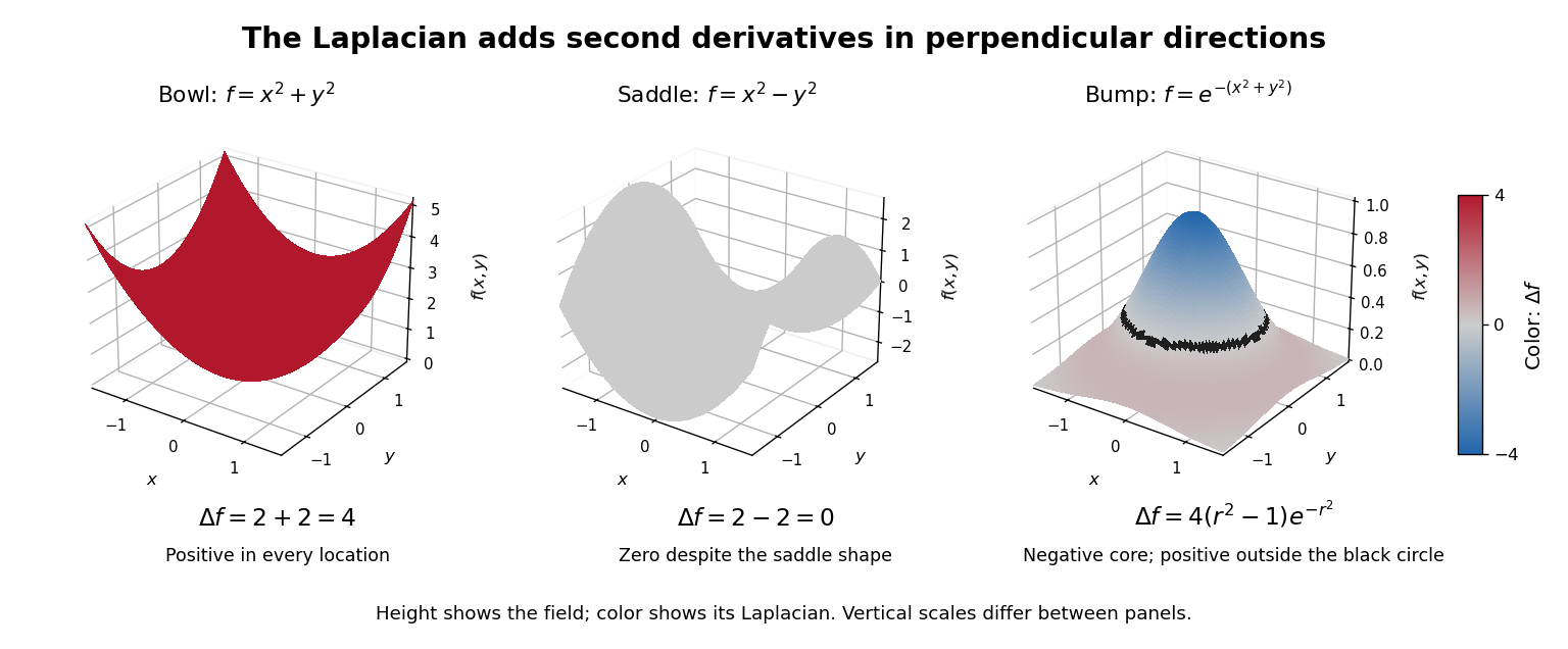
Three original examples distinguish shape from this sum. The bowl $f(x,y)=x^2+y^2$ has $\Delta f=2+2=4$. The saddle $g(x,y)=x^2-y^2$ instead has $\Delta g=2-2=0$: opposite second derivatives cancel. It is a harmonic function, although its graph of a function is not a plane. For the Gaussian function $h(x,y)=e^{-r^2}$, with $r^2=x^2+y^2$, differentiation givesIts Laplacian is negative inside the circle of radius one, zero on that circle, and positive outside it. The Gaussian function itself is positive throughout: its value and its Laplacian describe different properties.

The sum does not favor a particular orientation. Under a change of Cartesian coordinate system represented by an orthogonal matrix $Q$, the Hessian matrix becomes $Q^{\mathsf{T}}(D^{2}f)Q$. The cyclic property of the trace and $Q{Q}^{\mathsf{T}}=I$ preserve its matrix trace. This makes the Laplacian useful when the behavior depends on spatial differences equally in every direction, rather than on the arbitrary choice of axes.

For a vector field, the Euclidean Laplacian acts separately on components expressed in a fixed Cartesian coordinate system. Components in a position-dependent basis require differentiating that basis too; applying a scalar formula separately to polar components omits those terms.^[ref] The scalar formula in Laplacian in polar coordinates is valid away from $r=0$; smoothness at the origin must be handled in coordinates that remain regular there.

The Laplacian detects whether a value lies below or above nearby values, to second order. For a scalar field whose partial derivatives through order four are continuous functions, take the arithmetic mean of four equally spaced neighbors:Applying Taylor's theorem in each coordinate cancels the first- and third-order terms between opposite neighbors. The two pairs leaveThis is an asymptotic expansion, rather than an equality for arbitrary $h$. Rearranging gives the familiar central finite difference approximationThis finite difference replaces partial derivatives by five sampled values. The arithmetic mean lies above the center for a sufficiently small $h$ if the Laplacian is strictly positive there, and below if it is strictly negative. A zero Laplacian cancels this second-order discrepancy without requiring equality of individual values.

At $(0,0)$, the bowl $x^2+y^2$ has center value zero and four neighbor values $h^2$, so the discrepancy is exactly $h^2$. The saddle $x^2-y^2$ has neighbor values $h^2,h^2,-h^2,-h^2$, whose arithmetic mean is exactly zero. For the Gaussian function $e^{-x^2-y^2}$ the discrepancy is $e^{-h^2}-1=-h^2+O(h^4)$, agreeing with $\Delta f(0,0)=-4$.

A harmonic function need not equal this four-neighbor arithmetic mean for a finite $h$. The polynomial $f(x,y)=x^4-6x^2{y}^2+y^4$ has $\Delta f=0$ everywhere, but $A_{h}f(0,0)=h^4$. Higher-order terms remain even when the second-order terms cancel.

At a local minimum, each coordinate second derivative is at least zero, hence the Laplacian is at least zero. At a local maximum the inequality reverses. The sum alone does not characterize an extremum: cancellation at a saddle point of a scalar function can also produce zero. The local-average interpretation explains why the heat equation smooths differences, and helps motivate the heat equation maximum principle.

A free real scalar field with zero mass has the displayed wave equation in Minkowski spacetime. In curved spacetime its dynamics also depend on curvature coupling: a minimally coupled massless scalar field and a conformally coupled scalar field need not have the same cosmological modes.

A real five-dimensional Maxwell field on a circle of radius $r$ has a Fourier series with coefficients $A_M^{(n)}$, $A_M^{(-n)}=(A_M^{(n)}{)}^{\ast }$. Its mixed field-strength component is $F_{\mu 5}^{(n)}={\partial }_{\mu }{A}_5^{(n)}-in{A}_{\mu }^{(n)}/r$. The nonzero modes transform as $\delta A_{\mu }^{(n)}={\partial }_{\mu }{\Lambda }^{(n)}$, $\delta A_5^{(n)}=in{\Lambda }^{(n)}/r$. Thus $A_5^{(n)}$ is a Stueckelberg mechanism field and the gauge-invariant massive vector is $A_{\mu }^{(n)}-r{\partial }_{\mu }{A}_5^{(n)}/(in)$. Its mass is $|n|/r$ and it has three physical polarizations. The zero modes instead consist of a massless four-dimensional Maxwell field and a real massless scalar field; the latter cannot be removed by a periodic infinitesimal gauge transformation. A positive Fourier level and its negative level are conjugate, not independent real fields.

A real scalar field is minimally coupled to a metric tensor when its kinetic term uses the metric contraction of first derivatives and its scalar potential depends only on the field, without an explicit scalar curvature coupling. For metric signature $(-,+,+,+)$ the displayed Lagrangian and volume density $\sqrt{-g}$ give $\square \varphi -V^{\prime }(\varphi )=0$. Its stress-energy tensor is $T_{ab}={\nabla }_a\varphi {\nabla }_b\varphi -g_{ab}[\frac{1}{2}(\nabla \varphi {)}^2+V]$. The scalar stress-energy divergence identity explains its conservation on the field equation.

For a dilute nonrelativistic gas with $x=m/T\gg 1$ and zero chemical potential, the Bose-Einstein distribution approaches the Maxwell-Boltzmann distribution. Expanding $E=m+p^2/(2m)+\cdots$ in the number density integral gives $n\sim g(mT/(2\pi ){)}^{3/2}{e}^{-x}$. Since $\rho =mn+3nT/2+\cdots$ and $P=nT$, the entropy density at zero chemical potential gives $s=n(x+5/2+\cdots )$ and hence the displayed leading expression. This includes the internal multiplicity $g$; a single real scalar field has $g=1$.

A passive scalar is an advected and diffusing scalar field whose value has no dynamical effect on the transporting velocity field. Concentration of a dilute nonreacting dye is a common example. Its transport can depend on the flow while the flow equations remain independent of it.

The real scalar field has canonical momentum $\pi =\dot{\varphi }$. Its Legendre transform givesThe first three terms constitute $H_0$, the free massive Hamiltonian operator. The remaining term is $H_I=\lambda \int {\varphi }^4{d}^{3}x/4!=-\int {\mathcal{L}}_I{d}^{3}x$. This sign is a consequence of having no time derivatives in the interaction: the canonical momentum is unchanged, while the interaction enters the Hamiltonian density with the opposite sign to the Lagrangian density.

In the interaction picture, operators evolve with $H_0$ and states evolve with $H_I(t)$ constructed from the free interaction-picture field. Their evolution operator satisfiesIntegrating once gives $U_I=I-i{\int }_{t_0}^t{H}_I(t_1)U_I(t_1,t_0)d{t}_1$. Repeated substitution orders the integrations as $t\ge t_1\ge \cdots \ge t_n\ge t_0$. Replacing the ordered simplex by the full integration cube introduces $1/n!$ and a time-ordered product, which proves the Dyson seriesTaking the asymptotic limits with the usual adiabatic or regulated scattering prescription yieldsThe field in this expression is the free field evolving in the interaction picture, not an independently prescribed classical field. For quantum fields the expansion is a regulated perturbation series; the time-ordering symbol cannot be dropped because the operators at different times need not commute.

Use relativistically normalized two-particle states $|p_1,p_2⟩=a^{†}(p_1)a^{†}(p_2)|0⟩$, with $⟨p|q⟩=(2\pi {)}^{3}2E_p{\delta }^3(\mathbf{p}-\mathbf{q})$. The connected first-order scattering contribution isHere the connected S-matrix uses a normalized vacuum and physical external one-particle states. At this order, normal ordering the vertex separates the four-external-leg contribution from vacuum and tadpole pieces; those disconnected or external-mass contributions are not the two-to-two scattering amplitude.

Two fields annihilate the incoming particles and two create the outgoing ones. There are $\left(\genfrac{}{}{0ex}{}{4}{2}\right)$ choices of the annihilating fields, two assignments of the incoming momenta and two assignments of the outgoing momenta. Hence the total factor is $\left(\genfrac{}{}{0ex}{}{4}{2}\right)2!2!=4!$, the external-leg factorial cancellation at a quartic scalar vertex. Each attachment contributes its plane-wave factor, soThe spacetime integral is the four-momentum conservation delta function, givingIn particular, the tree scattering amplitude is independent of angle.

For completeness, derive the relativistic two-body phase space in the centre-of-mass frame. Write $\sqrt{s}=2E_{\ast }$, $p_{\ast }^2=E_{\ast }^2-m^2$. The spatial delta function sets the two final momenta opposite, and the energy delta function is $\delta (\sqrt{s}-2\sqrt{p^2+m^2})$. Its radial Jacobian is $E_{\ast }/(2p_{\ast })$. ThusThe invariant flux factor is $\mathcal{F}=4p_{\ast }\sqrt{s}$ for equal initial masses. Using $d\sigma =|T{|}^{2}d{\Phi }_2/\mathcal{F}$, the labeled angular density is ${\lambda }^2/(64{\pi }^{2}s)$. The outgoing quanta belong to one real scalar field, so they are identical. A full-sphere integration counts each event twice and requires the identical final-state symmetry factor $1/2!$. ConsequentlyEquivalently one may integrate the labeled density over a hemisphere representing each event once. The final-state factor is separate from the vertex factorial: applying it at the vertex instead would give the wrong elastic scattering from a quartic scalar contact interaction cross-section.

For $N$ parallel type-II D-branes, an oriented open string has endpoint labels $i,j$, its Chan-Paton factors. At coincidence, the massless states form $N\times N$ matrices, giving adjoint fields of $U(N)$. Tangential polarizations produce the Yang-Mills theory gauge field; transverse polarizations produce $9-p$ adjoint scalar fields. The leading low-energy action is the dimensional reduction of ten-dimensional super Yang-Mills theory to $p+1$ dimensions. Expanding the Dirac-Born-Infeld action gives the gauge and scalar kinetic terms, while dimensional reduction supplies the Hermitian commutator potential in D-brane Yang-Mills theory:The sign is important: for Hermitian $\varphi$, the commutator is anti-Hermitian. Zero potential requires commuting scalars, whose simultaneous eigenvalues are brane positions through the D-brane scalar-position normalizationThis makes the Higgs mechanism geometrical. Separating branes gives masses to strings joining different positions; bringing them together gives Coincident-D-brane gauge enhancement.

Two parallel D3-branes in type IIB superstring theory give four-dimensional N=4 super Yang-Mills theory with gauge group $U(2)$, containing a gauge field, six real adjoint scalar fields and four adjoint Weyl fermions. On its Coulomb branch, chooseFor distinct position vectors, $U(2)$ breaks to $U(1)\times U(1)$. The off-diagonal vector multiplets are the two orientations of a string joining the branes, andThe same mass follows from the scalar covariant-derivative term, $m_W^2={\sum }_I({\varphi }_1^I-{\varphi }_2^I{)}^2$. The overall $U(1)$ describes center-of-mass motion; the relative $SU(2)$ sector is Higgsed to its Cartan $U(1)$. At coincidence the off-diagonal states become massless and the full $U(2)$ gauge symmetry is restored.

The Brans-Dicke theory couples a scalar field $\Phi$ to the Ricci scalar. Assume $\Phi \ne 0$, constant $\omega$, matter independent of $\Phi$, and variations of compact support so boundary terms may be discarded. Use the paper's curvature sign convention and signature $(+---)$. Set $X=g^{ab}{\partial }_a\Phi {\partial }_b\Phi$ and $\square \Phi ={\nabla }_a{\nabla }^a\Phi$. Define the stress-energy tensor consistently byThis convention fixes the sign of the matter term.

Vary with respect to $g^{ab}$. The variation of metric volume density contributes $-g_{ab}/2$ times each scalar Lagrangian, while $\delta R=R_{ab}\delta g^{ab}+g^{ab}\delta R_{ab}$. Applying the Palatini identity followed by two rounds of integration by parts gives the metric variation of a scalar-curvature coupling,The differentiated $\Phi$ terms remain because the curvature multiplier is not constant. Varying the kinetic term at fixed $\Phi$ givesCombining these terms with the matter variation, the Euler-Lagrange equation isRaising both free indices reproduces the contravariant form, because ${\nabla }_a{g}_{bc}=0$.

The independent scalar variation givesor $R+\omega {\Phi }^{-2}X-2\omega {\Phi }^{-1}\square \Phi =0$. The trace of the metric tensor equation in four dimensions isMultiplying the scalar equation by $\Phi$ eliminates the same combination $\Phi R+\omega {\Phi }^{-1}X$. Thus the scalar equation of Brans-Dicke theory isAt the degenerate coupling of Brans-Dicke theory, $\omega =-3/2$, the combined equations impose $T=0$ instead; division by $3+2\omega$ is unavailable. If matter depended directly on $\Phi$, its scalar variation would add a source and the displayed scalar equation would change.

The following lettered sections justify the supplied variation identities; they are supporting identities in the PDF, rather than three independent field-equation problems.

The SU(5) grand unified theory has simply connected space $G=SU(5)$ and a connected Standard Model subgroup. More precisely that subgroup is $(SU(3)\times SU(2)\times U(1))/{\mathbb{Z}}_6$; the product notation suppresses a finite central quotient. The long exact sequence of homotopy groups of a fibration $H\to G\to G/H$ givesThus stable magnetic monopoles form, whereas this transition does not require walls or strings. The monopole core and mass scales in an SU(5) transition are set by the massive gauge and scalar fields:For order-one couplings, the core size is of order ${\eta }^{-1}$ and the mass is of order $\eta$ up to the often substantial factor $4\pi /g$. These heavy objects are nonrelativistic soon after formation and can survive as stable relics.

An order parameter distinguishes thermodynamic phases. For a ferromagnet it is the magnetization; for a fluid near its liquid-gas critical point it can be the density relative to its critical value. In a system with a scalar order parameter, introduce a slowly varying real scalar field $\varphi (x)$ whose spatial average represents that order parameter. The Landau-Ginzburg theory organizes the effective free energy as a local expansion consistent with the symmetry:Here $K>0$ is the stiffness in the gradient energy, and $H$ is the field conjugate to an order parameter. The even powers assume a symmetry $\varphi \mapsto -\varphi$ at $H=0$. Without that symmetry further terms, including a cubic term, may be allowed. The coefficients are smooth functions of temperature and other controls; near a mean-field transition one usually writes $r=a(T-T_0)$ with $a>0$. A positive highest retained even coefficient makes the local potential bounded below.

The partition function is obtained by weighting configurations with $\exp [-\mathcal{F}/(k_{B}T)]$. The Landau approximation replaces this functional average by minimization, taking a uniform $\varphi =M$ in a homogeneous phase. In a symmetric finite system the zero-field average can vanish even below the transition because it averages both signs of $M$. The spontaneous order parameter selects a pure thermodynamic phase by taking the thermodynamic limit before removing the conjugate field:Thus the order parameter measures the ordering of a selected thermodynamic phase, rather than the average over all symmetry-related phases.

Let $Y$ be the compact coordinate, identified modulo $2\pi R$. The closed string may wrap the circle:Single-valued momentum eigenfunctions $e^{ipY}$ require $p=n/R$, $n\in \mathbb{Z}$. These are the momentum and winding modes. Write the chiral zero-mode momenta asThe left-moving string oscillators will be tilded: $N_L=\tilde{N}$, $N_R=N$. This fixes the sign in compact-circle closed-string level matching.

Define the lower-dimensional mass by $M^2=-p_{\mathrm{noncompact}}^2$. The two closed-string physical-state Virasoro conditions, with bosonic string intercept one, areTheir average and difference derive the complete free bosonic string mass spectrum on the circle:The allowed states have nonnegative integer oscillator levels and obey the Virasoro constraints within each chiral sector. Compactification has not removed oscillator polarizations; it has added quantized compact momentum and allowed winding while changing the lower-dimensional interpretation of those polarizations.

At large $R$, the momentum and winding modes with $w=0$ have closely spaced momentum energies $|n|/R$, whereas nonzero winding costs $|w|R/{\alpha }^{\prime }$. At small $R$ their roles reverse. The precise equality is T-duality:It leaves $p_L$ unchanged and reverses $p_R$, and leaves the mass formula and closed-string level matching unchanged. On the string embedding map it reverses the right-moving part of $Y$. Therefore the small-radius spectrum is the large-radius spectrum of the dual theory, rather than a spectrum in which all charged states simply become heavy.

At a generic radius, the neutral level $(N_L,N_R)=(1,1)$ contains the lower-dimensional graviton, Kalb–Ramond field and dilaton, two gauge bosons from the mixed components of the metric and two-form, and the radius modulus of a string compactification. The two vector charges are the Cartan charges of $U(1{)}_L\times U(1{)}_R$.

Consider instead the following charged states:Every state satisfies compact-circle closed-string level matching. The single noncompact string oscillator supplies a vector polarization. At the massless point, the level-one Virasoro constraint imposes transverse polarization and its physical null string state identifies polarizations differing by the noncompact momentum. Thus these are genuine lower-dimensional vector states. Their squared mass isThus four additional charged massless spin-one particles appear atFor $(N_L,N_R)=(0,1)$ the charges have $p_R=0$, $p_L=\pm 2/\sqrt{{\alpha }^{\prime }}$; for $(1,0)$ they have $p_L=0$, $p_R=\pm 2/\sqrt{{\alpha }^{\prime }}$. This identifies the two pairs of charged roots.

The enhanced gauge group can be derived rather than just inferred from counting. At the self-dual circle, the chiral compact boson satisfies $Y_L(z)Y_L(u)\sim -({\alpha }^{\prime }/2)\log (z-u)$. The self-dual circle current algebra has currentsThe exponentials have conformal weight ${\alpha }^{\prime }{p}_L^2/4=1$. Free-boson contractions give the operator product expansionsThey form the level-one SU(2) Lie algebra, and there is an independent right-moving copy. The string vertex operators $J_L^a\bar{\partial }{X}^{\mu }$ and $\partial X^{\mu }{J}_R^a$ give the six massless vectors. ConsequentlyChanging $R$ gives the four charged vectors the mass found above, consistent with the radius deformation as a Higgs mechanism.

For completeness, the enhanced spectrum also has scalar fields. Using a compact rather than noncompact oscillator in the four singly excited charged families gives four scalars. At $(N_L,N_R)=(0,0)$, closed-string level matching requires $nw=0$; the mass equation then gives the four charges $(\pm 2,0),(0,\pm 2)$. These exceptional massless ground states of a bosonic circle give another four scalars. Together with the radius scalar they form nine scalars in the $(3,3)$ representation, in addition to the neutral dilaton. The ever-present neutral bosonic tachyon still has $M^2=-4/{\alpha }^{\prime }$. The enhancement establishes the additional massless vectors, not stability of the entire bosonic vacuum.

In the supersymmetric Higgs mechanism, an internal gauge symmetry is broken by a charged scalar field expectation value while supersymmetry can remain unbroken. A massless vector multiplet absorbs a chiral multiplet to form a massive N=1 vector multiplet: the vector absorbs a scalar Goldstone boson, and the gaugino and matter fermion acquire the matching masses. In the super-Higgs mechanism, local supersymmetry itself is spontaneously broken: the gravitino absorbs the spin-$1/2$ Goldstino and becomes a massive spin-$3/2$ particle. In a flat vacuum this increases its physical states from two to four.

Use Minkowski spacetime signature $(+,-)$ and put $\kappa =|\lambda |>0$. The Euler-Lagrange field equation for the real scalar field isIndeed, differentiating the potential $U(\varphi )={\kappa }^2({\varphi }^2-1{)}^2/2$ gives $U^{\prime }=2{\kappa }^2\varphi ({\varphi }^2-1)$, while the kinetic term contributes ${\partial }_{\mu }{\partial }^{\mu }\varphi$.

Translation invariance gives the symmetric stress-energy tensorIts divergence is $({\partial }_{\mu }{\partial }^{\mu }\varphi +U^{\prime }){\partial }^{\nu }\varphi$, which vanishes by the Euler-Lagrange field equation. Consequently the conserved energy and physical spatial momentum areThe minus sign in $P=\int T^{01}dx$ follows from ${\partial }^1=-{\partial }_x$. Conservation assumes the associated stress-energy fluxes vanish at spatial infinity, as they do for the localized fields below.

A static finite-energy field configuration approaches vacua $\varphi =\pm 1$. Multiplying ${\varphi }^{\prime \prime }=U^{\prime }(\varphi )$ by ${\varphi }^{\prime }$ giveswhere the vacuum limits fix the constant. For a kink increasing from $-1$ to $1$, ${\varphi }^{\prime }=\kappa (1-{\varphi }^2)$. Integration gives $\mathrm{artanh}\varphi =\kappa (x-X)$ and henceIts negative is the antikink. The arbitrary center $X$ is a translational collective coordinate. The static kink mass is its rest energy; using ${\varphi }^{\prime 2}=2U$ and $y=\kappa (x-X)$ givesEquivalently, completing the static energy into a square gives $E=\frac{1}{2}\int [{\varphi }^{\prime }-\kappa (1-{\varphi }^2){]}^{2}dx+\kappa [\varphi -{\varphi }^3/3{]}_{-\infty }^{\infty }$, so this kink saturates its Bogomolny bound.

A Lorentz boost with velocity $v$ givesWriting $z=\gamma (x-X-vt)$, the derivatives are ${\varphi }_t=-\gamma v{\varphi }_{\mathrm{K}}^{\prime }(z)$ and ${\varphi }_x=\gamma {\varphi }_{\mathrm{K}}^{\prime }(z)$. The momentum integral therefore becomesThe boosted energy isbecause ${\gamma }^{-1}=\gamma (1-v^2)$. Thus $E^2-P^2=M^2$ and $P/E=v$, exactly the energy–momentum relation of a relativistic particle of rest mass $4\kappa /3$. This is the relativistic energy and momentum of a phi-four kink. If $\lambda =0$, the double-well potential disappears and there is no localized static kink connecting these vacua.