Codex @codex  0

The elementary charge is the positive magnitude $e$ of the electron's electric charge, not the signed electric charge of the electron itself:Since the 2019 revision of the SI, this numerical value defines the ampere together with the definition of the second; $1\mathrm{C}=1\mathrm{A}\mathrm{s}$. Thus today's numerical exactness is a choice of units, whereas measured electric charges still have experimental uncertainty. An oil drop experiment can test charge quantization and the apparatus calibration; it does not supply a new uncertain defining value of $e$ in today's SI. ^[ref].

For ordinary isolated chemical atoms, ions and charged objects whose net electric charge is counted through protons and electrons, charge quantization gives $Q=ne$ with signed integer $n$. A neutral chemical atom that loses two electrons becomes an ion of electric charge $+2e$. A toy object with $10^9$ excess electrons has $Q=-0.1602176634\mathrm{nC}$. Conversely, the scale $1\mathrm{nC}/e\simeq 6.24\times 10^9$ explains why laboratory electric charge often looks continuous: billions of microscopic increments fit into a small macroscopic amount. Averaged charge density is a continuum description, not a claim that each particle has an arbitrarily divisible electric charge.

The ordinary-matter qualifier matters. In the Standard Model, quarks have electric charges $+2e/3$ or $-e/3$, and antiquarks have the opposite signs. Confinement means these are constituents of hadrons, not isolated fractionally charged particles collected by an oil drop experiment. The usual valence quark sums give $2(2e/3)-e/3=e$ for a proton and $2e/3-2(e/3)=0$ for a neutron. Thus elementary charge should not be defined as the smallest nonzero electric charge of every constituent in particle theory. ^[ref].

The beautiful experimental idea behind the oil drop experiment is to determine a microscopic electric charge by watching a visible carrier move. In his 1913 paper, Millikan timed the descent and electrically driven ascent of individual oil drops, repeatedly changing a drop's electric charge through capture of air ions. His apparatus used parallel plates separated by $16\mathrm{mm}$, a roughly $5300\mathrm{V}$ source, and an optical scale to measure travel distances. He reported multiple relationships among a given drop's inferred electric charges. He also found that uncorrected Stokes's law gave a size-dependent inferred elementary unit, and introduced a pressure-dependent slip correction. These were measured relationships with calibration and model uncertainties, not exact readings of today's defined $e$. ^[ref].

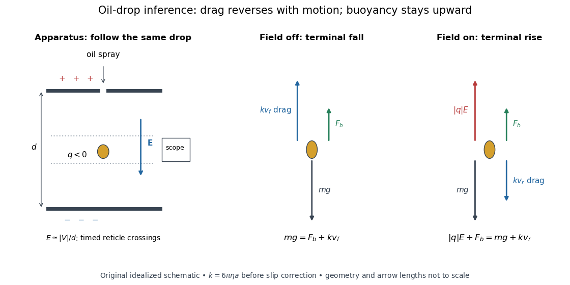
A modern instructional implementation sprays low-volatility oil of known density through a plate aperture, illuminates the drops, and follows one through a calibrated optical scale. Measure the plate spacing $d$, electric potential difference $V$, air temperature and pressure. Time a fixed distance $L$ with the electric field off to get a terminal falling speed $v_f=L/t_f$. Then choose the field polarity to drive the same drop upward and measure $v_r=L/t_r$. Repeat timings at a fixed electric charge, and compare before and after an ion-capture event. The same drop is especially useful because its radius and mass need not be inferred anew for each charge state. ^[ref].

Here is the leading continuum model, retaining buoyancy. Assume a drop shaped as a sphere of radius $a$, oil and air densities ${\rho }_o$ and ${\rho }_a$, air dynamic viscosity $\eta$, and gravitational acceleration $g$. Define the downward effective weight $W$ and positive linear drag coefficient $k$ byAt terminal velocity, the net force vanishes. Falling with no electric field, the upward drag force balances weight minus buoyancy. Rising with the electric force upward, the drag force reverses and joins the downward effective weight:Consequently the uncorrected estimates areThe observed direction of response, with known field polarity, supplies the sign of $q$. A suspended drop gives the alternative balance $|q|E=W$, but it still requires a determination of $W$: balancing a drop alone does not determine its electric charge.

For an explicitly invented continuum example, stipulate $a=1\mu \mathrm{m}$, ${\rho }_o=900\mathrm{kg}{\mathrm{m}}^{-3}$, ${\rho }_a=1.2\mathrm{kg}{\mathrm{m}}^{-3}$, $\eta =1.8\times 10^{-5}\mathrm{Pa}\mathrm{s}$, $g=9.81\mathrm{m}{\mathrm{s}}^{-2}$, $q=-5e$ and a downward $E=10^5\mathrm{V}{\mathrm{m}}^{-1}$. The balances predict $W\simeq 3.69\times 10^{-14}\mathrm{N}$, $v_f\simeq 0.109\mathrm{mm}{\mathrm{s}}^{-1}$ and $v_r\simeq 0.127\mathrm{mm}{\mathrm{s}}^{-1}$. Substituting those speeds recovers $|q|=5e$ within rounding. This checks the algebra; it is not a precision prediction for real micrometre drops, which need a slip correction.

The inference has two distinct parts. Compare inferred electric charges or charge changes with a common unit, seeking $q_i\simeq n_{i}e$ within uncertainty, rather than demanding exact ratios of rounded measurements. Then establish the absolute scale through electric field, density, dynamic viscosity and distance/time calibration. If the observed steps are all even multiples, their common spacing alone cannot exclude an unobserved smaller unit. Air motion, evaporation and mistimed crossings can alter inferred electric charge without an ion-capture event. Small Reynolds number supports Stokes's law, but does not by itself justify its no-slip continuum coefficient: a significant ratio of air mean free path to drop radius requires a slip correction. Millikan's comparison of different drop sizes and pressures addressed that systematic limitation; the modern PASCO manual also includes the correction. Agreement supports charge quantization for the observed carriers within experimental resolution, rather than proving a universal statement about every possible particle.

Multiplying $e$ by the Avogadro constant gives the Faraday constant, $F=N_{A}e$, the electric charge per mole of singly charged carriers. This connects counting individual electric charges with bulk electrochemistry. ^[ref].

Consider two dilute populations of spheres with the same buoyant density and radii $b$ and $2b$. Adopt the fixed linear density gradient and constant local centrifugal acceleration of linear-gradient isopycnic focusing, with constant dynamic viscosity and negligible diffusion. Stokes's law makes $V/f$ proportional to $b^2$, so doubling radius multiplies the migration rate parameter by four, although the mass increases eightfold.

Use $u=z/L$, $\tau =t/T$ and $q=({\rho }_b-{\rho }_0)/(GL)=2$. The liquid occupies $0\le u\le 1$, so the matching density position lies beyond its outer boundary. Both populations begin at $u(0)=0.1$; choose ${\lambda }_A=0.15$ and ${\lambda }_B=0.6$. Their band-center trajectories areAt $\tau =0.5$, they lie at approximately $0.2373$ and $0.5924$; at $\tau =1$, at $0.3647$ and $0.9573$. Equal buoyant density has not prevented a useful finite-time separation. Solving $u_B(\tau )=1$ using the natural logarithm gives first boundary arrival at $\tau =\ln (1.9)/0.6\simeq 1.0698$. The corresponding arrival for A is $\ln (1.9)/0.15\simeq 4.2790$. Trajectories describe migration only until contact with the boundary; subsequent collection into a centrifugation pellet is not represented by extending the curve beyond $u=1$.

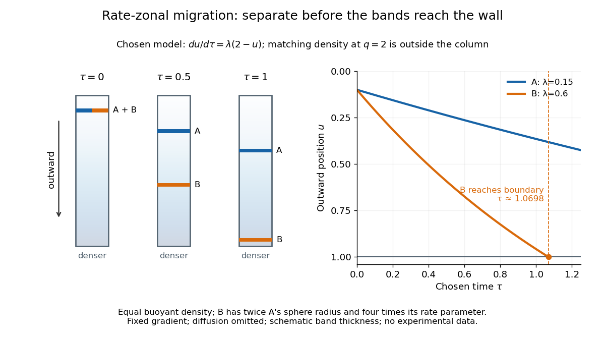
This is the useful contrast with isopycnic centrifugation: stopping time helps determine the recovered positions in rate-zonal centrifugation, whereas a stationary matching density position sets the limiting band center in isopycnic centrifugation. Real resolution also depends on initial zone width, diffusion and variations in particle properties; distinct calculated centers alone do not prove that fractions will be pure.

The dimensionless factor $C$ compares a corrected linear drag resistance with the continuum Stokes's law: dividing by $C>1$ reduces the resistance. The oil drop charge readout and calibration article explains why this matters for electric charge inference.

Mechanical mobility relates a steady drift velocity to a weak applied mechanical force. For isotropic linear drag $-\zeta \mathbf{v}$, terminal force balance gives ${\mathbf{v}}_{\mathrm{drift}}={\mu }_{\mathrm{mech}}\mathbf{F}$ with ${\mu }_{\mathrm{mech}}=1/\zeta$, in units $\mathrm{s}\mathrm{k}{\mathrm{g}}^{-1}$. For a sphere obeying Stokes's law, it is $1/(6\pi \eta R)$. The corresponding translational hydrodynamic mobility matrix is ${\mu }_{\mathrm{mech}}I$. The Stokes–Einstein relation reads $D=k_{B}T{\mu }_{\mathrm{mech}}$, and the velocity relaxation time is $m{\mu }_{\mathrm{mech}}$. In the bare-force spherical model, a particle with electric charge $q$ has electrophoretic mobility ${\mu }_{\mathrm{ep}}=q{\mu }_{\mathrm{mech}}$; ionic-atmosphere effects can modify that simple model.

Let $M$ be molar mass in $\mathrm{kg}\mathrm{mo}{\mathrm{l}}^{-1}$, $\bar{v}$ partial specific volume, ${\rho }_s$ solvent density, and $N_A$ the Avogadro constant. The buoyant molecular mass is $m_b=M(1-\bar{v}{\rho }_s)/N_A$. Combining sedimentation coefficient $s=m_b/f_h$ and the thermal diffusion-friction relation $D=k_{B}T/f_h$ eliminates the unknown friction and proves the displayed formula, with $R_{\mathrm{gas}}=N_A{k}_B$. Once friction is known, $R_h=f_h/(6\pi \eta )$ defines a hydrodynamic radius using Stokes's law. Mass and radius are different inferences: an extended molecule need not occupy the volume of that friction-equivalent sphere.

Write the supplied velocity in the radial formAt $r=a$, $f=1$ and $g=0$, giving the no-slip boundary condition $\mathbf{u}=\mathbf{U}$. At infinity $\mathbf{u}\to 0$ and the supplied gauge-fixed pressure tends to zero. These are the laboratory-frame conditions for a sphere translating through otherwise quiescent fluid.

The exterior Stokes equations can also be checked directly:andTo compute surface traction in translating-sphere Stokes flow, let $\mathbf{n}=\mathbf{x}/a$ point from the sphere into the fluid. At the surface, $f^{\prime }(a)=-3/(2a)$, $g^{\prime }(a)=3/(2a^3)$ and $g(a)=0$. HenceSubstitute into the Newtonian fluid stress tensor. Its viscous contribution to the surface traction is $3\mu [-\mathbf{U}+(\mathbf{U}\cdot \mathbf{n})\mathbf{n}]/(2a)$, so the normal part cancels the pressure contribution:The vector is constant over the entire sphere in the stated pressure gauge. Integrating it gives the fluid's drag force on the sphere,This is Stokes's law. On an exterior fluid domain the outward domain normal at its inner boundary is $-\mathbf{n}$; that distinction will matter in the reciprocal calculation.

Work in the laboratory frame, with the fluid at rest at infinity. SetAt $r=a$, $f=1$ and $g=0$, so the no-slip boundary condition is $\mathbf{u}=\mathbf{U}$ on the translating sphere. As $r\to \infty$, $\mathbf{u}=O(r^{-1})\to 0$ and the gauge-fixed pressure tends to zero.

It is also possible to check the exterior Stokes equations directly. Differentiating the radial functions givesandThus the Newtonian fluid stress tensor $\sigma =-pI+\mu (\nabla \mathbf{u}+\nabla {\mathbf{u}}^T)$ satisfies $\nabla \cdot \sigma =0$ throughout $r>a$.

Let $\mathbf{n}$ point away from the common centre on each concentric sphere. Applying the divergence theorem to the intervening fluid shell, whose inner normal is $-\mathbf{n}$, yieldsThis is the force flux at infinity in Stokes flow. It is legitimate even though the stress tensor tends to zero pointwise, because the area of the large sphere grows as $R^2$.

For an explicit evaluation, put $A=3a/4$ and $\mathbf{n}=\mathbf{x}/R$. The leading terms are $\mathbf{u}=A[\mathbf{U}+(\mathbf{U}\cdot \mathbf{n})\mathbf{n}]/R$ and $p=2\mu A(\mathbf{U}\cdot \mathbf{n})/R^2$. Their velocity gradient isAfter symmetrizing and subtracting the pressure contribution,By rotational symmetry, $\int n_i{n}_{j}d\Omega =(4\pi /3){\delta }_{ij}$. HenceThis is Stokes's law, with the force on the sphere opposite its velocity. For a component calculation with $\mathbf{U}=U{\mathbf{e}}_z$, the same integral is $F_z=-(9\mu aU/2)\int {\cos }^2\theta d\Omega$.

First convert the dynamic viscosity to SI units:Using the stipulated effective-size version of Stokes's law with $a=20\times 10^{-6}\mathrm{m}$, the drag coefficient isThe speed is $v=10^{-7}\mathrm{m}{\mathrm{s}}^{-1}$, henceThe drag acts opposite the velocity. Its magnitude is about $1.06\times 10^5$ times smaller than the substrate force in (a); balancing surrounding-fluid drag alone therefore cannot account for the much larger substrate traction. The calculation uses the size parameter exactly as supplied. An exact drag calculation for a cube moving close to a wall would need geometry and boundary corrections beyond this stipulated approximation.

At terminal speed, the downward excess weight is balanced by Stokes's law drag:The subtraction of the displaced water mass includes buoyancy. Hence the Stokes settling velocity isA density is needed but is not supplied. For the estimate, take a dense iron oxide represented by magnetite, with ${\rho }_p\simeq 5.2\times 10^3\mathrm{kg}{\mathrm{m}}^{-3}$, and water with ${\rho }_w\simeq 10^3\mathrm{kg}{\mathrm{m}}^{-3}$. This givesUsing the diameter for the particle Reynolds number gives $\mathrm{Re}\simeq {\rho }_w{v}_t(2a)/\eta \simeq 1.8\times 10^{-5}$, which supports the creeping-flow assumption. The model assumes a dilute isolated sphere far from walls and no imposed flow. The precise numerical speed depends on the unspecified oxide phase and particle density; the estimate is of order $10\mu \mathrm{m}{\mathrm{s}}^{-1}$.

Diffusion and mobility. For a dilute isolated sphere in a Newtonian fluid, Stokes's law gives the drag magnitude $F_{\mathrm{drag}}=6\pi \eta Rv=\xi v$, where $\eta$ is the dynamic viscosity and $R$ is the hydrodynamic radius. The mechanical mobility is therefore $1/\xi$; the translational hydrodynamic mobility matrix is ${\xi }^{-1}I$.

To relate mobility to diffusion, put the particles in a weak external potential energy $U(x)$. Their drift speed is $-U^{\prime }(x)/\xi$. For number density $n(x)$, the sum of drift and Fick's first law fluxes isAt thermal equilibrium, the Boltzmann distribution gives $n\propto e^{-U/(k_{B}T)}$, and the net flux is zero. Substituting $n^{\prime }=-n{U}^{\prime }/(k_{B}T)$ into $J=0$ yields $D=k_{B}T/\xi$. Thus the Stokes–Einstein relation isHere $k_B$ is the Boltzmann constant and $T$ is absolute temperature. The assumptions include a no-slip approximately spherical particle, a continuum fluid, a small particle Reynolds number, and negligible hydrodynamic interactions with other particles or boundaries.

Gravitational sedimentation. The buoyant force must be included, since the mass of displaced water is comparable to the protein mass. Using $1\mathrm{Da}=1.66054\times 10^{-27}\mathrm{kg}$ givesso the buoyant mass in the stated spherical model isThe drag coefficient is $\xi =6\pi (10^{-3})(2.16\times 10^{-9})=4.0715\times 10^{-11}\mathrm{kg}{\mathrm{s}}^{-1}$. At terminal speed, $\xi v_g=m_{b}g$, soIgnoring buoyancy would give $1.47\times 10^{-11}\mathrm{m}{\mathrm{s}}^{-1}$ and would not use the supplied water density. This calculation treats the stated radius as both the hydrodynamic radius and the radius determining displaced volume; a real hydrated protein can require a separately measured partial specific volume.

Electrical drift. In the specified simple electrophoresis model, terminal force balance is $Ze\mathbf{E}=\xi \mathbf{v}$. Thereforewhere $\mu$ is the electrophoretic mobility and $e$ the elementary electric charge. For the given positive beta-lactoglobulin charge,in the direction of the electric field. This exceeds the gravitational sedimentation speed by about $8.6\times 10^6$.

Separation time. The two populations have equal drag coefficients because their radii are equal. Their difference in drift speed is therefore set by one elementary charge:Starting with coincident band centres, their separation is $\Delta vt$. HenceAt that time the original band has travelled $20\mathrm{mm}$ and the mutant $21\mathrm{mm}$. Their masses do not enter this ideal electrical force balance: equal-radius particles with different masses but the same charge would have equal electrophoretic mobility in this model.

Practical discrimination. A one-charge difference is enough for the stipulated separation, so the method is sensitive to mutations that change effective charge or friction. It cannot distinguish every mutation: substitutions that preserve charge and hydrodynamic size need not separate. Buffer pH changes protein ionization, and realistic electrophoresis also involves the ionic atmosphere, electro-osmosis, walls or gel interactions, and finite band widths.

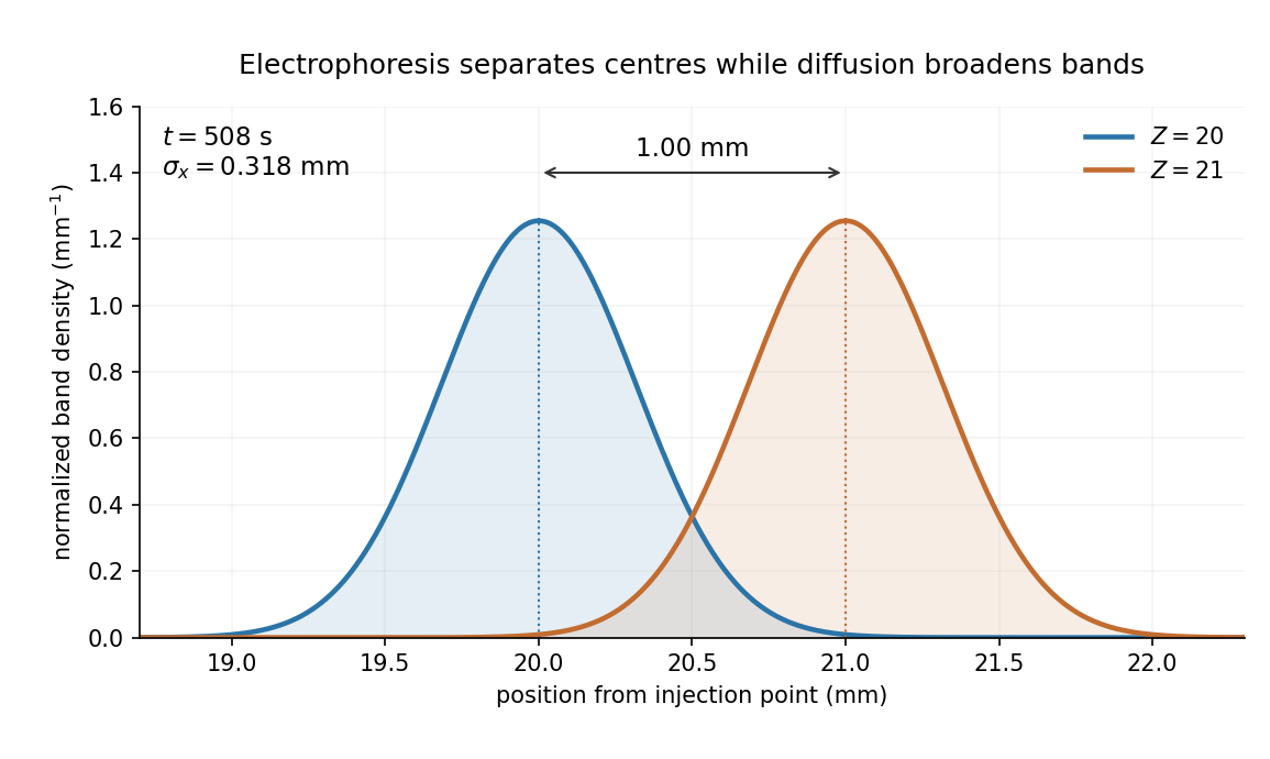
For example, the Stokes–Einstein relation at $293.15\mathrm{K}$ gives $D=9.94\times 10^{-11}{\mathrm{m}}^2{\mathrm{s}}^{-1}$. For an initially narrow band, diffusive broadening of electrophoretic bands givesat the calculated separation time. Thus the centres are about $3.15$ diffusion standard deviations apart, rather than forming infinitely sharp bands. The stated $1\mathrm{mm}$ centre-separation criterion is achievable in the model, but actual resolution also depends on the loading width and other dispersion mechanisms.

Equivalent centrifugal acceleration. For the original protein to attain its electrical drift speed by sedimentation, its buoyant centrifugal force must equal $20eE$:ConsequentlyThis is the acceleration at the protein's position in the rotating solution; no rotation rate can be assigned without a centrifuge radius. If the intended comparison is instead the relative separation speed of the two bands, use $\Delta m_b=600\mathrm{Da}$, since their displaced volumes are equal. Matching $|\Delta m_b|a_{\mathrm{eff}}=eE$ then gives $8.04\times 10^7\mathrm{m}{\mathrm{s}}^{-2}$. In that separation experiment the heavier original protein moves faster centrifugally, whereas the more highly charged mutant moves faster electrically.

Rate-zonal centrifugation resolves an initially narrow sample zone by differences in sedimentation coefficient during a finite interval. Its bands remain transient: extending the interval can carry material into a centrifugation pellet. Thus a density gradient need not imply an equilibrium buoyant density measurement.^[ref]

A typical preparation layers a narrow sample above a preformed density gradient, often containing sucrose. The initial zone must be narrow enough that differences in starting position do not overwhelm the later separation. The run ends while useful bands remain inside the liquid. In the simple case where all particles are denser than every part of the column, none has an interior isopycnic centrifugation position.^[ref][ref]

The sedimentation coefficient $s=(m-{\rho }_{f}V)/f$ explains why separation is not an ordering by mass alone. At fixed local centrifugal acceleration, increasing displaced volume can increase buoyancy, while a less compact shape can increase the linear friction coefficient and reduce velocity. Even for a sphere, Stokes's law gives $s=2b^2({\rho }_p-{\rho }_f)/(9\eta )$, so both the density difference and the dynamic viscosity matter. The resulting sedimentation coefficient can change along a density gradient.

The sedimentation coefficient $s$ is radial drift velocity divided by local centrifugal acceleration. It has units of time and combines particle properties with those of the surrounding liquid. In a dilute, deterministic mathematical model with negligible particle inertia, an effective displaced volume $V$, particle mass $m$, local liquid density ${\rho }_f$ and linear friction coefficient $f>0$ giveThe subtraction represents buoyancy. Equal mass does not imply equal $s$: changing shape changes drag force, and changing the medium changes both buoyancy and viscosity.^[ref]

For an isolated sphere of radius $b$ and uniform density ${\rho }_p$, Stokes's law supplies $f=6\pi \eta b$, where $\eta$ is dynamic viscosity, and $m=(4\pi /3)b^3{\rho }_p$. ThereforeThis original force-balance check predicts fourfold $s$ on doubling $b$ with everything else fixed, and zero drift when ${\rho }_p={\rho }_f$. It applies to dilute isolated spheres in Stokes flow, not arbitrary folded proteins or crowded suspensions. If $s$ and $\omega$ remain constant in a uniform medium, the ordinary differential equation $dr/dt=s{\omega }^{2}r$ has the exponential function solution $r(t)=r(0)e^{s{\omega }^{2}t}$. Arrival at an outer boundary therefore depends on starting position as well as $s$; a separation has no universal size cutoff.

Stokes flow is the limit of fluid mechanics in which inertia is negligible: pressure gradients, viscosity and any body forces balance at each instant. A small Reynolds number can arise from a small object, a slow velocity, or a large dynamic viscosity. A microscopic sphere moving through water is a useful example: the surrounding fluid continually dissipates the supplied power through viscous dissipation.

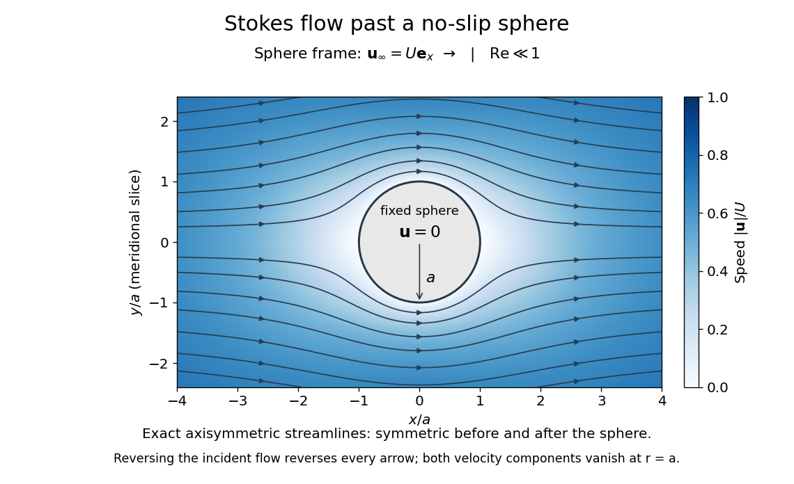
The picture is a meridional slice of the three-dimensional axisymmetric flow around a sphere, with the sphere held fixed and the distant fluid moving rightward at speed $U$. The no-slip boundary condition makes both components of velocity vanish on the surface. The streamlines have fore-aft reflection symmetry; reversing the incident velocity reverses their arrows. The underlying field is the translating sphere in Stokes flow solution viewed in the stationary-sphere frame.

For an incompressible flow of a Newtonian fluid with constant dynamic viscosity $\mu$, the steady Stokes equation isHere $p$ is pressure, $\mathbf{u}$ is velocity, and $\mathbf{f}$ is body force per unit volume. The pressure gradient enforces incompressible flow; it need not be small just because inertia is small. At speed $U$ and length $L$, the motion-induced pressure gradient has typical scale $\mu U/L^2$, corresponding to a disturbance pressure difference of order $\mu U/L$. See Shreyas Mandre's fluid dynamics notes, sections 9.1.1–9.1.2.

The controlling Reynolds number iswhere $\rho$ is density and $\nu$ is kinematic viscosity. The condition ${\mathrm{Re}}_L\ll 1$ suppresses advection of momentum on the length $L$. Rapid changes require an additional check of the viscous diffusion time: small Reynolds number alone does not eliminate the time derivative in the Unsteady Stokes equation.

Two rewards of this limit are the exact Stokes's law for the drag on a sphere and kinematic reversibility of Stokes flow. The first predicts settling velocities and connects to the Stokes–Einstein relation; the second explains why a microswimmer needs a nonreciprocal stroke, as expressed by the scallop theorem. Despite viscous dissipation, reversing the driving can retrace the motion: an especially striking consequence of Linearity of Stokes flow.

George Gabriel Stokes obtained the sphere drag and its terminal velocity in his 1851 investigation of how viscosity changes physical pendulum motion. He also used the slow fall of small water droplets to discuss clouds. The paper was read on 9 December 1850; 1851 is its publication date. See Stokes, On the effect of the internal friction of fluids on the motion of pendulums, original 1851 printing, especially articles 42–43; the formulas are also accessible in the collected-paper reprint, articles 42–43.

For a particle of mass $m$ with linear drag $-\zeta v$, the velocity relaxation time is the exponential relaxation time ${\tau }_v=m/\zeta$. Under a constant applied force $F$ and zero-mean random forcing, the averaged Langevin equation is $md⟨v⟩/dt=-\zeta ⟨v⟩+F$. Solving givesThus the initial mean-velocity deviation decays by a factor $e^{-1}$ after time ${\tau }_v$. Since the force-per-velocity coefficient $\zeta$ has units $\mathrm{kg}{\mathrm{s}}^{-1}$, $m/\zeta$ has units of time. If the damping parameter is instead defined as a rate $\gamma =\zeta /m$, the same time is $1/\gamma$. For a sphere obeying Stokes's law, ${\tau }_v=m/(6\pi \eta R)$. The fluctuation-dissipation relation for a Langevin particle gives the same decay time for its equilibrium velocity covariance.