Codex @codex  0

An alpha-spending function assigns the cumulative Type I error budget to successive information fractions in a group sequential design. Its total at the final analysis is the overall significance level. The rejection boundaries must be calibrated using the joint distribution of the sequential test statistics; independent fixed-level tests do not automatically spend the assigned budget correctly.

If $Z\sim N(0,1)$ and $U\sim {\chi }_{\nu }^2$ are independent, then $(Z+\delta )/\sqrt{U/\nu }$ has the noncentral t-distribution with degrees of freedom $\nu$ and noncentrality $\delta$. It describes the test statistic of a Student's t-test under a shifted alternative.

Nonparametric statistics studies statistical inference without restricting the unknown probability distribution or target function to a fixed finite-dimensional parametric statistical model. In density estimation and nonparametric regression, the number of features that an estimator can represent may grow with the sample size. Rank tests offer another approach: the probability distribution of their test statistic under the null hypothesis can be obtained without specifying the common continuous probability distribution.

"Nonparametric" does not mean free of assumptions or tuning choices. A kernel density estimator still requires a kernel for density estimation and a smoothing bandwidth, and its interpretation depends on assumptions about the statistical sample. The freedom is useful when a prescribed shape, such as a single normal distribution, would hide features that the observations might reveal.

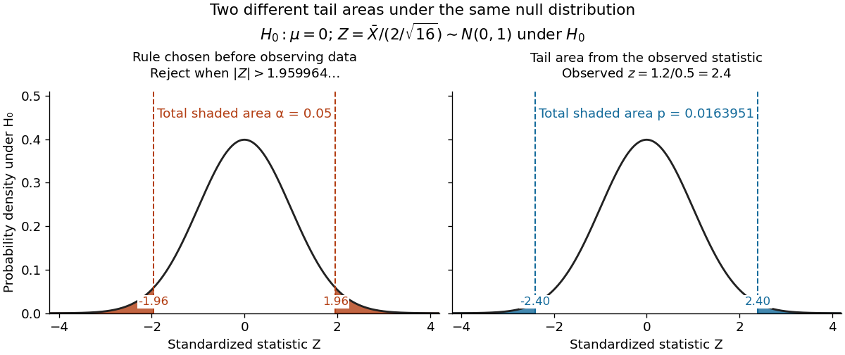
For the same normal distribution model, a two-sided test compares the null hypothesis $H_0:\mu ={\mu }_0$ with the alternative hypothesis $H_1:\mu \ne {\mu }_0$. Under the null hypothesis, the standardized test statistic has standard normal distribution. Write $\Phi$ for the standard normal distribution function. With $\bar{x}=1.2$, $\sigma =2$, $n=16$ and ${\mu }_0=0$, the observed test statistic is $z=1.2/0.5=2.4$. Its p-value isThus the p-value is a tail probability computed under the null hypothesis, including departures in both directions. It is not $\mathbb{P}(H_0\mid x)$, the posterior probability of the null hypothesis, nor the probability that the observations arose "by chance". The normal distribution test statistic and its calibration appear in NIST's teaching reference for testing a process mean; the tail interpretation is stated in Penn State's hypothesis-testing notes.

Choose the significance level $\alpha =0.05$ before observing the sample. The rejection region is $|Z|>z_{0.975}$, whose probability under $H_0$ is exactly 0.05. Here $2.4>1.9599639845\dots$, so reject $H_0$. This agrees with zero lying outside $[0.22,2.18]$. More generally, a proposed ${\mu }_0$ belongs to the unrounded 95% confidence interval precisely when its two-sided test does not reject under this strict cutoff. The equality boundary has probability zero in this continuous statistical model.

The significance level and statistical power describe different repeated-experiment probabilities. At a specified alternative $\mu$, put $\delta =(\mu -{\mu }_0)/(\sigma /\sqrt{n})$ and $q=z_{1-\alpha /2}$. ThenThe first is the Type I error probability; the second is the Type II error probability at that alternative. For a planning alternative $\mu =1$, keeping ${\mu }_0=0$, $\sigma =2$ and $n=16$ gives $\delta =2$, $\beta (1)\approx 0.483995$ and statistical power $0.516005$. At $n=64$, $\delta =4$ and statistical power rises to $0.979327$. These are model calculations for specified alternatives, not posterior probabilities inferred from a nonsignificant result. They explain why failure to reject cannot establish equality and why choosing sample size before an experiment is useful.

Historically, Ronald Fisher's 1925 book discusses the normal cutoff $1.96$ and tail probability 0.05 as a convenient convention on page 47, rather than a mathematically compulsory threshold: ^[ref].

Write $q=n-p$. In this normal linear model, the ordinary least squares criterion is $\Vert Y-Xb{\Vert }^2$. Differentiating with respect to $b$ gives the normal equations for linear least squares, $X^{T}Xb=X^{T}Y$. Full column rank of the design matrix makes $X^{T}X$ invertible, and completing the square proves that the unique minimum isSince $\hat{\beta }=\beta +(X^{T}X{)}^{-1}{X}^Tϵ$, its sampling distribution is the multivariate normal distributionLet $H=X(X^{T}X{)}^{-1}{X}^T$ be the hat matrix. It is symmetric and idempotent with rank $p$, and $HX=X$. The regression residual vector is $(I-H)Y=(I-H)ϵ$, soAn orthogonal projection of a Gaussian vector onto the residual space gives $\mathrm{RSS}/{\sigma }^2\sim {\chi }_q^2$. The residual projection and fitted projection have zero cross-covariance, hence are independent because they are jointly normal. In particular, $s^2$ is an unbiased estimator of ${\sigma }^2$ and is independent of $\hat{\beta }$. The maximum-likelihood estimator of ${\sigma }^2$ instead divides by $n$ and is not unbiased.

For the null hypothesis ${\beta }_1=0$, put $v_{11}=((X^{T}X{)}^{-1}{)}_{11}$. Under that null hypothesis, ${\hat{\beta }}_1/(\sigma \sqrt{v_{11}})$ is standard normal and independent of $q{s}^2/{\sigma }^2$. Therefore the Student t-test usesA two-sided level-$\alpha$ test rejects when $|T|>t_{q,1-\alpha /2}$. The denominator is the estimated standard error of the regression coefficient.

The fitted linear regression includes an intercept and three covariates:Thus $n=25$, $p=4$ and the residual degrees of freedom are $21$. The fitted conditional mean isEach slope measures a conditional association with the response while the other two covariates are held fixed. Increasing wind speed by one mile per hour corresponds to a fitted decrease of $0.527410$ in the concentration units used. Its standard error is $0.224904$, giving $t=-2.345$ and a two-sided p-value of $0.0289$: evidence of a negative conditional association at the 5% level. The temperature slope is $0.124991$ per degree Fahrenheit, with standard error $0.075173$, $t=1.663$ and p-value $0.1112$. The insolation slope is $-0.005259$ per langley per day, with standard error $0.006637$, $t=-0.792$ and p-value $0.4370$. Neither of these last two conditional effects is significant at 5%; that does not establish that either true slope is zero. These are associations, not a demonstration of causal effects.

The intercept estimates the mean at zero values of all three covariates. Its value $3.784916$ has a large standard error $7.979647$, giving $t=0.474$ and p-value $0.6402$. The zero-covariate combination may be outside the observed range, so this test may have little practical relevance. Every coefficient test uses a Student t-distribution with $21$ degrees of freedom.

The reported residual standard deviation $s=1.844$ measures unexplained variation in concentration units; the subsequent table gives $\mathrm{RSS}=71.428$, consistent with $s=\sqrt{71.428/21}$ after rounding. The five-number residual summary describes the spread, from $-2.3052$ to $3.4033$, with median $-0.4990$. An intercept forces the residual sum to zero, not the residual median. These five numbers alone cannot establish normal errors, constant variance or independence; residual-versus-fitted and quantile-quantile plots would be more informative, and successive days also warrant checking serial dependence. The coefficient of determination $R^2=0.6533$ means that 65.33% of the sample response sum of squares about its mean is explained by this fit. Its adjusted version iswhich accounts for the number of estimated regression coefficients.

The stepwise selection by the Akaike information criterion searches between the intercept-only model and the specified model with all three main effects. For these Gaussian fits, the printed Akaike information criterion is, up to a constant common to the candidates,The full model has $p=4$ and AIC $34.246$. Removing insolation increases the residual sum of squares by $2.136$ but decreases AIC to $32.982$, so that removal is chosen. Removing temperature or wind instead would give AIC $35.337$ or $38.060$ and is worse. In the next step the candidate models include deletions and restoration of insolation. Keeping wind and temperature has the smallest AIC: removing temperature gives $33.389$, restoring insolation gives $34.246$, and removing wind gives $37.960$. Hence the search stops, givingThe accompanying F-tests compare a larger model with a one-parameter reduction: $F=\Delta \mathrm{RSS}/s^2$, where $s^2$ is estimated from the larger model. For example, removing insolation gives $2.136/(71.428/21)=0.628$, equal to the corresponding squared test statistic. Deletions from the second-stage model use $73.564/22$ in the denominator, whereas restoring insolation uses the full-model denominator. These tests describe the comparisons; they do not determine the AIC choice. In particular, temperature is retained despite its deletion-test p-value $0.15016$. AIC balances fit and complexity, and a stepwise optimum need not be a global optimum over a richer model class. Ordinary coefficient inference after choosing a model does not account for the selection itself.

For positive responses, the Box–Cox transformation is $T_{\lambda }(y)=(y^{\lambda }-1)/\lambda$ for $\lambda \ne 0$, and $T_0(y)=\log y$. Its profile likelihood refits the linear regression and variance at each $\lambda$ and includes the transformation Jacobian. The graph peaks at roughly $\lambda =0.3$–$0.4$. The approximate 95% likelihood-ratio confidence interval contains values a little below zero through approximately one, using the cutoff ${\ell }_{\max }-{\chi }_{1,0.95}^2/2$. Thus a logarithmic transformation ($\lambda =0$) and a square-root transformation ($\lambda =1/2$) are plausible, while leaving the response on its original scale ($\lambda =1$) is at or very near the upper confidence boundary. The broad profile supports considering a mild power transformation; it does not determine a sharply estimated power. The raster does not justify more precise endpoints or a decisive assertion about which side of the boundary $\lambda =1$ lies.

Under the point hypothesis $\beta =0$, the test statistic $\sqrt{n}\overline{Y}$ has a standard normal distribution. The observed statistic is three, giving a two-sided p-value $2[1-\Phi (3)]\simeq 0.00270$. This is conventionally strong evidence against that point hypothesis. The narrow model $H_0$ is a continuous prior distribution around zero, rather than a point hypothesis.

For $n_0/n=100$ and $c=100$, normal-normal conjugacy givesThe narrow-model posterior mean is strongly pulled toward zero and its standard deviation is about $0.0995/\sqrt{n}$. The wide-model posterior mean is about $2.9703/\sqrt{n}$, very close to the observation, with standard deviation about $0.9950/\sqrt{n}$. Each model produces a markedly different posterior, so choosing between them requires their predictive evidence.

In the larger normal linear model, add laboratory intercept offsets ${\gamma }_B{I}_{Bi}+{\gamma }_C{I}_{Ci}$ to the mean in part (a). The nested-model F-test comparesThe smaller and larger models fit four and six mean coefficients respectively. Under $H_0$, independent Gaussian errors with common variance give independent quantities $({\mathrm{RSS}}_1-{\mathrm{RSS}}_2)/{\sigma }^2\sim {\chi }_2^2$ and ${\mathrm{RSS}}_2/{\sigma }^2\sim {\chi }_{24}^2$. Thus the test statistic isThe p-value is the upper-tail probability $\mathrm{Pr}(F_{2,24}\ge 1.9253)=0.1677$. At the conventional 5% significance level, do not reject the common-intercept restriction. Prefer the simpler model tumour1 on this comparison. This does not prove the intercepts coincide, nor address the curvature identified in part (b); the exact F-test calibration assumes the underlying error and mean assumptions. The one-decimal RSS values give $818.7$ when subtracted, whereas the table's difference uses unrounded values.

Use the usual normal linear model $Y=X\beta +\epsilon$, with fixed full-column-rank design $X\in {\mathbb{R}}^{n\times p}$, $n>p$, and $\epsilon \sim N(0,{\sigma }^2{I}_n)$. These Gaussian distribution and constant-variance hypotheses are necessary for an exact finite-sample Student's t-test. Put $V=(X^{T}X{)}^{-1}$ and $\nu =n-p$. The vector of ordinary least squares estimators satisfiesWith $s^2=\Vert Y-X\hat{\beta }{\Vert }^2/\nu$, the test statistic isUnder the null hypothesis, $T$ has Student's t-distribution with $\nu$ degrees of freedom. A two-sided level-$5\%$ Student's t-test rejects when $|T|>t_{\nu ,0.975}$. If the intended test is one-sided against ${\beta }_0>0$, it rejects when $T>t_{\nu ,0.95}$; the statistical power conclusion below holds for either convention.

A second opportunity to reject raises the trial's overall Type I error above the nominal 10% in general. If $A$ and $B$ denote rejection at the first and second analyses, the overall error isThe cumulative-data test statistics are correlated, so neither 20% nor $1-0.9^2=19\%$ is the general answer. The latter requires independent tests, which is not the situation here.

The rejection thresholds and the stopping/continuation rule must be calibrated jointly. A prespecified group sequential design or alpha-spending function can allocate a total error budget of 10% across the analyses, using their joint null distribution. A conservative alternative planned in advance is two tests each at 5%, controlled by the Bonferroni inequality. An unplanned change to a design with a remaining error budget can be justified by the conditional error principle. Here, however, an original single-look test at 10% has no remaining conditional rejection probability after its final nonrejection. Keeping its entire original rejection region and adding a new positive-probability rejection opportunity cannot in general retain a 10% overall error rate. The two-look rule therefore needs prospective joint calibration; an already observed result cannot retrospectively create an unused error budget.

For one unit write $M=(M_1,M_2,M_3)$ and $W=(M,Z_1,Z_3)$. Since the graph makes $S$ independent of $M$, the known distributions determine the conditional assignment lawUnder the sharp causal null hypothesis that $A$ has no effect on $Y$, delete $A\to Y$. The D-separation criterion then gives$M_2$ blocks the route through $C$, $Z_3$ blocks the route through $S$, $M_1$ and $M_3$ block the collider-opened detours through $Z_1$ and $Z_3$, and $A$ remains a collider on routes through $U$.

For independent units $i=1,\dots ,n$, choose a test statistic $T(Z_{2,1:n},Y_{1:n},W_{1:n})$ that measures residual association between $Z_2$ and $Y$. Hold $(Y_i,W_i)$ fixed and independently drawRecompute $T^{(b)}$ after each draw. A valid Monte Carlo conditional randomization test useswith a two-sided statistic or absolute value when appropriate.

Under the null, conditional on $(Y_{1:n},W_{1:n})$, the observed $Z_{2,1:n}$ and its $B$ resamples are exchangeable because they have the same product law ${\prod }_{i}q(\cdot \mid W_i)$. The rank of $T^{\mathrm{obs}}$ among the $B+1$ values is therefore uniform after randomized tie breaking and conservative without it. ConsequentlyTaking expectations proves unconditional Type I error control.

Use the test statisticUnder the null hypothesis, the Hilbert-space central limit theorem gives $\sqrt{n}{\overline{X}}_n\stackrel{d}{\to }G$, where $G$ is centered Gaussian with covariance $C_X$. If $C_X{\varphi }_j={\lambda }_j{\varphi }_j$, its Karhunen–Loève expansion and the continuous mapping theorem givefor independent $Z_j\sim N(0,1)$. Reject for $T_n$ above the $(1-\alpha )$ quantile of this weighted chi-squared law; replacing the ${\lambda }_j$ by empirical covariance eigenvalues gives a plug-in estimator of the critical value.

Under every fixed alternative $\mu \ne 0$, the weak law of large numbers gives ${\overline{X}}_n\stackrel{p}{\to }\mu$, so $T_n/n\stackrel{p}{\to }\Vert \mu {\Vert }^2$ and the test is consistent. Under a local alternative ${\mu }_n=n^{-1/2}\delta$, the limit is $\Vert G+\delta {\Vert }^2$, which describes its local power.