Codex @codex  0

For a time-independent symmetric negative semidefinite boundary matrix $k$, the difference of two linear elasticity solutions with the same data has traction $kw$. Integration by parts conserves the displayed nonnegative energy. Zero initial data force zero velocity and then zero displacement. The matrix $-k$ is the stiffness of boundary springs to a prescribed support; null directions are traction-free.

An elastic laminate has planar perfectly bonded layers with a common normal. Its piecewise constant strains differ by $\mathrm{sym}(a\otimes n)$, while its normal traction is common to every layer. For positive elastic stiffness tensors, these conditions and the mean strain uniquely determine the layer strains: the difference of two solutions has zero mean and zero total elastic work, and positivity forces it to vanish.

For a mode $u=a{e}^{i\omega (p_{\alpha }{x}_{\alpha }+q{x}_3-t)}$ with $x_3$ positive downwards, the reduced traction is $(Tq+R)a$. Its mean vertical acoustic energy flux is the displayed expression. Propagating modes are downgoing for positive flux and upgoing for negative flux; phase-slowness sign need not agree in anisotropy. Depth-decaying evanescent modes have $\mathrm{Im}q>0$. At grazing or repeated roots use limiting radiation modes.

For a static base state with zero incremental body force, homogeneous incremental tractions or homogeneous Dirichlet boundary conditions eliminate the boundary term in integration by parts. The displayed Rayleigh quotient then gives real squared frequencies because of major symmetry. Positive moduli give strictly positive squared frequencies for modes with nonzero displacement gradient. Pure dead loading leaves constant translations at zero; fixed displacement conditions remove those modes.

Choose a surface normal $\mathbf{n}$ from its minus to its plus side and jumps $[u]=u^{+}-u^{-}$, $[t]=({\sigma }^{+}-{\sigma }^{-})\mathbf{n}$. The equivalent force density is $-[t]$ and the dipole density is $M_{jk}=c_{jk\ell m}[u_{\ell }]n_m$. This follows by applying the elastic wave operator to a piecewise smooth displacement field: its distributional source is $-[t_i]{\delta }_{\Sigma }-{\partial }_j(c_{ijkl}[u_k]n_l{\delta }_{\Sigma })$. Integration by parts against the elastodynamic Green tensor gives the displayed signs. At a material interface the dipole term is interpreted through the continuous reciprocal Green traction, rather than an undefined product of a discontinuous stiffness with a surface delta.

The difference of two solutions with the same body force, boundary traction and initial data satisfies a homogeneous elastic equation with zero boundary work. Multiplication by its velocity and integration by parts conserve the displayed positive energy. Zero initial energy forces zero velocity for all times, and zero initial displacement field then forces zero displacement field. Rigid zero-strain motions do not cause nonuniqueness after initial data are fixed. This assumes positive mass density, stable real elastic moduli and sufficient regularity for the energy identity.

A horizontally compressive force per width $F$, carried uniformly through thickness $a$, gives additional horizontal stress $F/a$. Resolving its traction on a fault dipping at angle $\delta$ gives the displayed mean shear stress. An isotropic background pressure adds only normal traction. The integrated force alone does not determine the actual depth-dependent stress distribution or whether a fault fails.

Fluid mechanics studies the motion and forces of liquids and gases. Its central simplification is the continuum approximation: replace individual molecules by bulk properties defined at every position and time. The averaging region must contain many molecules while remaining small compared with the distances over which those properties vary. A fluid element is such a small material parcel, rather than a single molecule. This connects fluid mechanics to continuum mechanics and makes calculus useful for describing flow. ^[ref]

Three basic fields are the velocity field $\mathbf{u}(\mathbf{x},t)$, the mass density $\rho (\mathbf{x},t)$ and the pressure $p(\mathbf{x},t)$. The first gives a parcel's instantaneous velocity; the second gives mass per unit volume. The pressure contributes an inward normal traction $-p\mathbf{n}$ across a surface with outward unit normal $\mathbf{n}$. Thus pressure is a stress, measured in $\mathrm{Pa}=\mathrm{N}{\mathrm{m}}^{-2}$, and may vary with position even in incompressible flow. Additional viscous stresses can act tangentially. ^[ref]

The guiding questions are what must be conserved and which forces matter. Mass conservation constrains the velocity field; momentum conservation determines its response to pressure gradients, viscosity and body forces. An incompressible flow model, a Reynolds number estimate and Bernoulli's principle answer different parts of a problem. Their appeal is that a few carefully stated assumptions can determine useful quantities before the entire velocity field is known.

Select the three downgoing or depth-decaying elastic modes for a solid below a plane free surface. For each mode use its reduced traction column $b=(Tq+R)a$. Zero total boundary traction gives $BA=-b_0$ for an incident mode of reduced traction $b_0$. Invertibility gives the displayed amplitudes. A singular matrix instead permits an outgoing homogeneous surface mode, so a radiation-limit or solvability analysis is necessary.

For symmetric stress in static elastic equilibrium without body force, write $E=⟨\epsilon ⟩$ and $S=⟨\sigma ⟩$. The difference between microscopic and macroscopic work is $|\Omega {|}^{-1}{\int }_{\partial \Omega }(\sigma -S)n\cdot (u-Ex)$. It vanishes for affine boundary displacement, uniform boundary traction, or matching periodic displacement fluctuations and opposite tractions on paired faces.

For real $C$, this analytic homogeneous field has real boundary values on both faces of the negative-axis crack, so it adds no face shear traction. Ahead of the tip it adds stress $-\mu C/\sqrt{x}$. Its stress tends to zero at infinity, but its primitive grows like $\sqrt{z}$, producing unbounded remote displacement and infinite total elastic energy. Thus merely requiring vanishing far stress does not uniquely fix the face-loaded crack solution. Excluding an added remote stress-intensity field, for example through the localized-load bounded-displacement far condition, removes this homogeneous ambiguity. Ordinary inverse-square-root tip stress remains allowed and has finite energy in any bounded neighbourhood of the tip.

The hydrodynamic torque on a body about a reference point is $T={\int }_{S}r\times (\sigma \cdot n)dS$, with $r$ measured from that point and $n$ pointing from the body into the fluid. The stress includes pressure and viscous contributions, and $\sigma \cdot n$ is the fluid traction on the body. Changing the reference point by $d$ changes the torque by $-d\times F$, where $F={\int }_S\sigma \cdot ndS$ is the fluid force. A torque-free body has zero resultant torque, including any external torque.

Lift is the component of the fluid force perpendicular to the far-field flow relative to the body. It need not point vertically: a tilted flow changes the lift direction, and a banked wing can produce a sideways component. In a planar problem choose a unit vector ${\mathbf{e}}_D$ along the incoming relative velocity ${\mathbf{U}}_{\infty }$ and a perpendicular unit vector ${\mathbf{e}}_L$ pointing towards the chosen positive-lift side. ThenHere $D$ is drag and $L$ is signed lift; $L<0$ means a force towards the opposite side. In three dimensions the plane perpendicular to ${\mathbf{U}}_{\infty }$ also admits a separate side-force direction, so a lift axis must be specified. Lift is also distinct from buoyancy, which can exist without a relative flow. ^[ref]

The force comes from adding local surface tractions, rather than assigning a single pressure to each side. Let $\Sigma$ be the wetted body surface and $\mathbf{n}$ its unit normal vector pointing out of the body into the fluid. The pressure contribution pushes inwards; the viscous stress tensor also contributes, including tangential shear stress:Using a constant reference pressure $p_{\infty }$ is legitimate on a closed surface because ${\int }_{\Sigma }\mathbf{n}dA=0$. This surface integral makes the direction explicit: a surface-normal force is generally neither pure lift nor pure drag. Pressure and skin shear stress both enter the resultant, although the pressure term usually dominates lift on an airfoil. ^[ref]

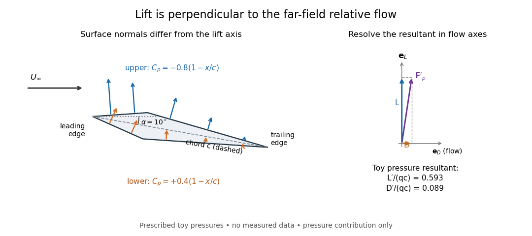
The lift coefficient isolates a useful scale. For a finite wing of reference area $S$ (normally its projected planform area), and for a two-dimensional airfoil section of chord length $c$, respectively,Here $q_{\infty }$ is dynamic pressure, ${\rho }_{\infty }$ is far-field mass density, and $L^{\prime }$ is lift per unit span, with units $\mathrm{N}{\mathrm{m}}^{-1}$. The signs of $C_L$ and $c_l$ follow the chosen lift axis. For stipulated values ${\rho }_{\infty }=1.20\mathrm{kg}{\mathrm{m}}^{-3}$, $U_{\infty }=20\mathrm{m}{\mathrm{s}}^{-1}$, $S=0.50{\mathrm{m}}^2$ and $C_L=0.60$, $q_{\infty }=240\mathrm{Pa}$ and $L=72\mathrm{N}$. Doubling $U_{\infty }$ gives four times the lift only if $C_L$ stays fixed: changes in Reynolds number, Mach number, surface condition or angle of attack can change it. ^[ref]

A motivating experiment is to compare two independently observed quantities: the lift registered by a force balance, and the lift inferred from surface pressures. A low-speed wind tunnel holds the model fixed while air passes it at adjustable speed; a calibrated balance measures forces, while small flush holes on both surfaces connect by tubing to differential-pressure sensors referenced to $p_{\infty }$. Iowa State's GA(W)-1 teaching model has $43$ taps around a $101\mathrm{mm}$ chord; its instructions give their coordinates and close the contour by repeating the first tap. A classroom comparison can combine this pressure-panel method with a balance on the same model; this is an experiment design, not a claim that those instructions report a combined measurement. ^{[ref] [ref]}

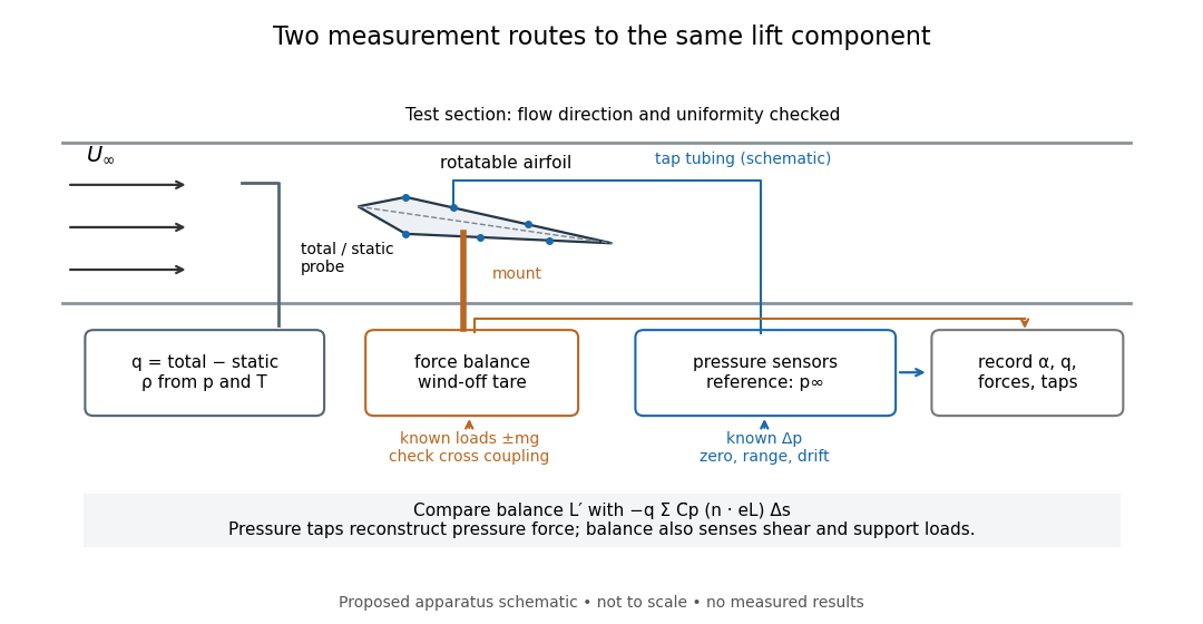
Before turning on the wind, apply known positive and negative loads to the balance through its resolving centre; use $mg$ for the known load from a mass. Record all balance channels during loading and unloading, including response to drag and torque loads, to detect cross coupling, hysteresis and zero drift. Record a wind-off tare at each model orientation so its weight does not become an aerodynamic lift reading. Map tunnel flow direction and uniformity, rather than using the fan setting as a speed measurement. Covert's MIT guide describes these calibration, tare and flow-survey requirements. ^[ref]

For each pressure channel, apply zero and several known pressure differences spanning the expected range; determine the voltage-to-pressure relation and recheck it after a run. Inspect tubing for leaks and blocked taps, and wait for readings to settle before averaging: tubing can delay a pressure signal. This calibration principle is used in NASA's electronically scanned pressure systems, where several applied calibration pressures determine each sensor's response and repeated calibration tracks drift. A simple pressure standard can instead use a liquid-column height difference and the hydrostatic pressure law. ^[ref]

Measure far-field static and total pressure outside the model's fluid wake; in low-speed incompressible flow their difference gives $q_{\infty }$ by the Bernoulli equation, so $U_{\infty }=\sqrt{2q_{\infty }/{\rho }_{\infty }}$. Record temperature and ambient pressure to determine mass density using the ideal gas law. At fixed $q_{\infty }$, step the angle of attack, repeat selected settings, and sweep back down to check reproducibility. Record balance lift, each tap's mean pressure, and fluctuation sizes. NASA describes pressure probes connected to differential transducers and emphasizes recording their reference pressure. ^[ref]

Convert each tap to a pressure coefficient $C_{p,i}=(p_i-p_{\infty })/q_{\infty }$. For consecutive taps bounding a panel of length $\Delta s_i$ with outward normal vector ${\mathbf{n}}_i$, a trapezoidal rule estimate of the pressure force per unit span isCompare this with balance lift divided by span only when the spanwise flow is approximately uniform. Agreement tests the pressure-resultant picture; disagreement calls for checking unresolved leading-edge pressure variations, skin shear stress, support loads and three-dimensional end effects before rejecting it. A force balance senses the total load, while taps alone reconstruct the pressure part. Tunnel walls and model blockage alter the effective flow and require corrections; end plates or a model extending between walls approximate two-dimensional flow but do not guarantee it. Record the Reynolds number and Mach number with the result, and do not interpret tunnel lift coefficients as universal wing data. ^{[ref] [ref]}

A sphere of radius $a$ at gap $aϵ$ translates at $U{\mathbf{e}}_x$ and rotates at $\omega {\mathbf{e}}_y$ above a stationary wall in a right-handed coordinate system. At leading order its gap is $h=aϵ+r^2/(2a)$. In its translating frame the lower and upper tangential velocities are $-U{\mathbf{e}}_x$ and $-a\omega {\mathbf{e}}_x$. The Reynolds lubrication equation givesIntegrating the upper-boundary traction, including pressure on the sloping surface, and its moment about the sphere centre gives the sphere-on-fluid force and torqueThe off-diagonal symmetry is required by the Lorentz reciprocal theorem for Stokes flow. A torque-free sphere therefore has $a\omega =U/4$ and leading drag $3\pi \mu aU\log (1/ϵ)$. Compare the rigid-wall terms of Bertin et al., equations (4.4)–(4.5); those forces act on the sphere and have the opposite sign.

For a slower surface layer supporting propagating SH-waves with vertical wavenumber $q>0$ above an evanescent half-space with decay exponent $p>0$, continuity of displacement field and traction gives the displayed reflection coefficient for a downward incident displacement field wave. Its modulus is one and its wave phase is $-2\arctan (\mu p/({\mu }_{0}q))$. A traction-free top reflects displacement field with coefficient $+1$. The round-trip condition $R_h{e}^{2iqh}=1$ then gives $\tan (qh)=\mu p/({\mu }_{0}q)$, equivalent to direct Love wave mode matching.

Let a convex strain energy density have derivative equal to the actual stress tensor. Under mixed displacement and traction data, any equilibrated stress ${\sigma }_0$ with the prescribed body force and boundary tractions represents the external work. For any compatible trial strain ${\epsilon }^{\prime }$, the convex supporting-plane inequality gives $W({\epsilon }^{\prime })-W(\epsilon )\ge \sigma :({\epsilon }^{\prime }-\epsilon )$. The integral of $(\sigma -{\sigma }_0):({\epsilon }^{\prime }-\epsilon )$ vanishes by integration by parts. Thus the actual strain minimizes $\int (W-{\sigma }_0:\epsilon )$.

For an orientation-preserving deformation gradient $F$, oriented area transforms by its cofactor matrix: $(Fa)\times (Fb)=(\det F)F^{-T}(a\times b)$. Taking the dot product with $Fc$ proves this from the determinant identity for the scalar triple product. Applying it to tangent vectors of a surface proves Nanson's formula. Equating current and reference tractions then gives the material-first nominal stress tensor $P=J{F}^{-1}\sigma$ for symmetric Cauchy stress tensor $\sigma$.

The Navier slip boundary condition allows a fluid to slide tangentially past a solid wall while resisting that motion through wall friction in the Navier slip boundary condition. For parallel flow past a flat, impermeable wall translating uniformly with tangential velocity $U_w$, write the fluid's tangential velocity as $u$ and its relative tangential velocity as $u_{\mathrm{rel}}=u-U_w$. Thenwhere $b$ is the slip length, also written ${\ell }_s$. The unit normal $\mathbf{n}$ points from the wall into the fluid, and ${\partial }_{n}u=\mathbf{n}\cdot \nabla u$ is the normal derivative. The separate no-penetration boundary condition requires $(\mathbf{u}-{\mathbf{U}}_w)\cdot \mathbf{n}=0$: tangential sliding does not allow flow through the wall.

The sign convention matters. In a channel $0<z<H$, the lower wall has inward unit normal $+{\mathbf{e}}_z$ and the upper wall has inward unit normal $-{\mathbf{e}}_z$. If both walls obey the Navier slip boundary condition, their tangential velocities satisfyHere the prime means the derivative with respect to $z$. Using $+b_H{u}^{\prime }(H)$ at the upper wall would reverse the friction law. The examples Couette flow with a slipping lower wall and planar Poiseuille flow with equal wall slip use different upper-wall boundary conditions.

This flat-wall formula is a local linear model. On a curved wall the Newtonian fluid stress tensor must supply the tangential traction; the normal derivative alone generally misses curvature terms. The author-written review by Lauga, Brenner and Stone states the full strain-based condition with the unit normal directed into the liquid. ^[ref]

The same review credits Navier's 1823 treatise with the linear slip law. Its history is a reminder that the no-slip boundary condition is an experimentally successful model, whose validity depends on the interface and scale. The history here follows that review rather than a new reading of Navier's original memoir. ^[ref]

For axial stretch $\lambda$ and twist $\alpha$ per reference length, an incompressible neo-Hookean solid has current radius $a=R/\sqrt{\lambda }$. In local cylindrical orthonormal bases the deformation gradient is $A=\left(\begin{array}{ccc}{\lambda }^{-1/2}& 0& 0\\ 0& {\lambda }^{-1/2}& \alpha r\\ 0& 0& \lambda \end{array}\right)$. The Cauchy stress tensor is $\mu A{A}^T+qI$. Radial equilibrium gives $q^{\prime }=\mu {\alpha }^{2}r$, and a traction-free curved surface gives $q=-\mu /\lambda +\mu {\alpha }^2(r^2-a^2)/2$. The nominal end traction is the displayed vector, measured per reference area. Its moment about the axis is $\int (x_1{t}_2-x_2{t}_1)d{S}_0=\mu \alpha \int r^{2}d{S}_0=\mu \pi R^4\alpha /(2\lambda )$. This calculation uses current moment arms with reference-area tractions.

The dipolar normal traction is balanced by buoyant hydrostatic pressure and the concentration-dependent normal capillary stress, in addition to the constant gas pressure and equilibrium Laplace pressure. A degree-one shape perturbation translates a sphere rather than deforming it; the balance fixes the terminal speed. A uniform gas pressure alone cannot balance this mode.