Codex @codex  0

For the equal-cardinality basis criterion, because $S$ spans $V$, repeatedly remove a vector whenever it is a linear combination of the others. Such a removal does not change the span. The finite process ends with a linearly independent spanning subset $T$, hence a basis of $V$.

If the original $S$ were linearly dependent, at least one removal would occur and $|T|<n$. But a basis of an $n$-dimensional vector space has $n$ vectors. Equivalently, apply the allowed claim to the basis $T$ and any fixed $n$-vector basis of $V$: the latter would wrongly be linearly dependent. Thus no removal was possible. The original spanning set is linearly independent and therefore a basis.

Writing the given bases as $(u_1,\dots ,u_p)$ and $(v_1,\dots ,v_q)$, a basis of the Cartesian product with its componentwise vector space operations isThis is the direct sum basis. Therefore $\dim (W_1\times W_2)=p+q=\dim W_1+\dim W_2$. The construction includes zero-dimensional factors, whose corresponding portion of the basis is empty.

Let $E_{ij}$ denote a matrix unit, with its only nonzero entry equal to one in row $i$, column $j$. A basis for the vector space of real skew-symmetric matrices isEach upper-triangular entry is free, its reflected lower-triangular entry is its negative, and every diagonal entry is zero. This is the basis of the space of real skew-symmetric matrices.

Regard $A$ as a linear map ${\mathbb{R}}^4\to {\mathbb{R}}^4$. By the rank-nullity theorem and matrix rank $3$,All three are vector subspaces of ${\mathbb{R}}^4$, with the row space identified with four-component row vectors in the usual way. The null space lies in the input vector space of concentrations; the column space lies in the output vector space of concentration-change rates. Both have four coordinates, although they play different physical roles.

In this particular matrix, the row sums and column sums both vanish. Put $1=(1,1,1,1{)}^T$. Then $A1=0$ and $1^{T}A=0$, and the two three-dimensional vector subspaces coincide:This equality follows here from both sum identities and the dimensions of a vector space; it does not make $A$ a symmetric matrix and is not true for every square matrix.

The identity and the three Pauli matrices form an orthogonal basis for the complex vector space of two-by-two matrices, with Hilbert-Schmidt inner product $\mathrm{Tr}(P^{†}Q)=2{\delta }_{PQ}$. Thus every operator has the expansion $A=\frac{1}{2}{\sum }_{P\in \{I,X,Y,Z\}}\mathrm{Tr}(PA)P$. For a density matrix, the identity coefficient is $1/2$ and the remaining real coefficients are half the components of its Bloch vector. This converts unitary conjugation into transformations of three real components.

Four projective points in general linear position in the complex projective plane impose four independent linear conditions on the six coefficients of a quadratic polynomial. To see independence, put them at the three coordinate points and $[1:1:1]$ using a projective frame. The remaining equations are $Axy+Bxz+Cyz=0$ with $A+B+C=0$, a two-dimensional vector space. Projectivizing its nonzero elements gives a pencil. It has nonsingular bases, for example the forms with coefficient triples $(1,1,-2)$ and $(1,-2,1)$, because the determinant of the symmetric coefficient matrix is $ABC/4$. Its three singular members are exactly the three pairs of lines obtained by partitioning the four base points into two pairs.

For finite-dimensional vector spaces $V,W$ over a field $F$, a bilinear pairing $B:V\times W\to F$ is perfect when the induced linear maps $V\to W^{\ast }$ and $W\to V^{\ast }$ are isomorphisms. Equivalently, both dimensions agree and the matrix of the pairing in any two bases is invertible. The evaluation pairing between a finite-dimensional vector space and its dual space is perfect. This notion allows two different spaces; a nondegenerate bilinear form is the case $V=W$.

The Petrov-Galerkin method chooses an approximate solution $u_h$ in a finite-dimensional trial vector space $V_h$ and tests a weak formulation against a possibly different test space $W_h$. For a bilinear form $a$ and a linear functional $\ell$, it imposes $a(u_h,v_h)=\ell (v_h)$ for every $v_h\in W_h$. Taking $W_h=V_h$ recovers the usual Galerkin method. Different test functions can alter stability and accuracy; the Galerkin orthogonality is then against the test space and need not be an orthogonal projection in an energy norm.

For an ordered basis $(x_i)$ of a Lie algebra $\mathfrak{g}$, the ordered monomials $x_1^{a_1}\cdots x_n^{a_n}$ form a basis of $U(\mathfrak{g})$. In particular, a triangular decomposition $\mathfrak{g}={\mathfrak{n}}^{-}\oplus \mathfrak{t}\oplus {\mathfrak{n}}^{+}$ gives $U(\mathfrak{g})\cong U({\mathfrak{n}}^{-})\otimes U(\mathfrak{t})\otimes U({\mathfrak{n}}^{+})$ as vector spaces.

For functions $f,g:X\to V$ taking values in the same vector space, pointwise addition is defined by $(f+g)(x)=f(x)+g(x)$ for every $x\in X$. For $f(x)=x$ and $g(x)=x^2$, the resulting function is $x\mapsto x+x^2$; at $x=2$ its value is six.

The zero function and pointwise scalar multiplication make the collection of all such functions a vector space. The vector space identities follow by evaluating at an arbitrary input and using the corresponding identities in $V$. This construction also preserves continuity and linearity when the original functions have those properties, and is the addition used in the superposition principle for a linear differential equation.

A Poisson algebra has two compatible products on one vector space: a commutative, associative multiplication and a Lie bracket $\{f,g\}$. Compatibility is the Leibniz ruleThus fixing $f$ makes $g\mapsto \{f,g\}$ an algebraic derivation. The Lie bracket also satisfies the Jacobi identity; an arbitrary bilinear bracket satisfying antisymmetry of a Lie bracket and the product rule need not do so.^[ref]

For example, the polynomial ring $\mathbb{R}[q,p]$ becomes a Poisson algebra with the canonical Poisson bracketThe partial derivatives give $\{q,p\}=1$ and $\{q,p^2\}=2p$, illustrating how the Leibniz rule extends the bracket from generators to their products. More generally, smooth functions on a symplectic manifold form a Poisson algebra. A finite-dimensional Lie algebra of moment map components need not be closed under ordinary multiplication: adding all their products normally gives a much larger Poisson algebra.

Polynomial evaluation replaces the indeterminate of a polynomial by an input value. For a fixed scalar $a$, the rule $E_a:p\mapsto p(a)$ is a linear functional on a vector space of polynomials, because evaluating a linear combination gives the same linear combination of the values. For $p(t)=1+2t+3t^2$, evaluation at zero gives one and evaluation at two gives seventeen. Polynomial interpolation uses these measurements to reconstruct a polynomial subject to a polynomial degree bound.

A linear operator $T:V\to V$ on a vector space over a field $k$ makes $V$ a module over the polynomial ring $k[t]$: let $t$ act as $T$, let constants act as the original scalars, and define $p(t)\cdot v=p(T)v$. The identity $(pq)(T)=p(T)q(T)$ for polynomials $p,q$ verifies the multiplication axiom. The submodules are precisely the invariant subspaces of $T$. This construction is described in Keith Conrad's Introductory Notes on Modules, section 6.

For a computed example, take $k=\mathbb{Q}$, $V=k^2$, andThen $T{e}_2=e_1$, $T{e}_1=0$, and $T^2=0$. ConsequentlyEvery $(a,b)$ equals $(b+at)\cdot e_2$. The module homomorphism $k[t]\to V$, $p\mapsto p(T)e_2$, is therefore surjective, and its kernel is the ideal $(t^2)$. It induces a module isomorphism $V\cong k[t]/(t^2)$. This is a cyclic module and a torsion module over $k[t]$, since $t^{2}V=0$. Over $k$ it is a free module with basis $(e_1,e_2)$ and has no nonzero torsion elements of a module. Over $\mathbb{Q}$ its nonzero elements also have infinite additive order of a group element. Changing scalars changes the questions one asks about the same addition law.

A polynomial moment functional is a linear functional on polynomials defined by their integrals against a specified function. For example, suppose the required integrals exist and setFor a polynomial $p(t)={\sum }_{j=0}^n{c}_j{t}^j$, linearity givesThus the finitely many moments ${\mu }_0,\dots ,{\mu }_n$ determine $L$ on the vector space of polynomials of degree at most $n$. Existence of these moments is part of the hypothesis; an arbitrary choice of $w$ need not give finite integrals.

For example, take $w=1$ on $[-1,1]$. Then ${\mu }_j=0$ for odd $j$ and ${\mu }_j=2/(j+1)$ for even $j$. On quadratic polynomials,The zero first moment records cancellation of the odd function $t$ on a symmetric interval. This finite-coordinate viewpoint is useful in Gaussian quadrature: a weighted sum of point evaluation functionals integrates every polynomial up to degree $n$ exactly if it agrees with $L$ on the monomials $1,t,\dots ,t^n$.

The real polynomials of degree at most $k$, together with the zero polynomial, form a vector space of dimension $k+1$ with basis $1,x,\dots ,x^k$. Polynomial spaces of lower degree are nested vector subspaces.

A convex polytope is the convex hull of finitely many points in a finite-dimensional real vector space. Equivalently, it is a bounded intersection of finitely many closed half-spaces. Its affine dimension may be smaller than that of the ambient space. Broader uses of polytope, including abstract or nonconvex versions, must specify their convention.

The simplex is the convex hull of affinely independent points; a square is a two-dimensional polytope with four vertices. The cube $[0,1{]}^n$ can be described either by its $2^n$ vertices or by the inequalities $0\le x_i\le 1$. These are its vertex and half-space descriptions.

A linear objective on a nonempty polytope attains its maximum at some vertex: every point is a convex combination of vertices, and its objective value is the same combination of vertex values. This links the geometry to linear programming. The maximizing vertex need not be unique, and an entire face may attain the optimum.

A linear map between ordered vector spaces is positive if it carries the positive cone of the domain into the positive cone of the codomain. For function spaces this means $f\ge 0⟹Tf\ge 0$. A Feller semigroup consists of such positive maps on continuous functions.

A tied largest modulus can prevent even direction convergence. With $D=\mathrm{diag}(2,-2)$ and $x_0=(1,1{)}^T/\sqrt{2}$,The two directions form a cycle; neither is an eigenvector. There is no dominant-modulus spectral gap. A tied modulus is not a universal failure: an initial eigenvector remains on its line, and $A=2I$ preserves every direction. Subspace iteration addresses a separated cluster by targeting a dominant invariant subspace instead of one eigenvector.

An orthogonal start can fail despite a strict spectral gap. For $A=\left(\begin{array}{cc}2& 1\\ 1& 2\end{array}\right)$ and $x_0=(1,-1{)}^T/\sqrt{2}$, the dominant component is zero, so $A{x}_0=x_0$ and every iterate equals $x_0$. The Rayleigh quotient is exactly $1$ and the eigenpair residual is zero, although the dominant eigenvalue is $3$. Exact arithmetic never creates a missing component.^[ref]

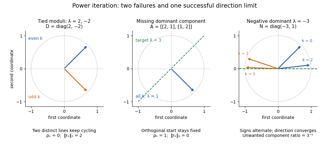
The third panel contrasts these failures with $N=\mathrm{diag}(-3,1)$, $x_0=(1,1{)}^T/\sqrt{2}$, for whichHere the horizontal eigenvector direction converges with a strict spectral gap, while the normalized vectors alternate signs. This is the successful direction convergence described under sign and phase in power iteration.

For a nonorthogonal eigenbasis, even the word “orthogonal” must be used carefully. The diagonalizable matrix $C=\left(\begin{array}{cc}3& 2\\ 0& 1\end{array}\right)$ has right eigenvectors $v_1=(1,0{)}^T$, $v_2=(-1,1{)}^T$, and dominant left eigenvector $w_1=(1,1{)}^T$. For $x_0=(a,b{)}^T$, the dominant coefficient is $c_1=w_1^T{x}_0=a+b$. The starting vector $v_2$ is nonorthogonal to $v_1$ but stays at the smaller eigenvalue $1$; $(0,1{)}^T$ is orthogonal to $v_1$ but has $c_1=1$ and converges to the dominant direction. The left eigenvector test, not the right-eigenvector inner product, controls the outcome.

A random vector drawn from a continuous probability distribution with a probability density function on the full real or complex vector space has $c_1\ne 0$ with probability one. This avoids the exact missing-component hyperplane, but does not guarantee a large component or fast convergence. Floating-point arithmetic may seed a missing component, yet a structurally preserved zero can remain zero, so accidental perturbations are not a convergence guarantee.

Let $Kx=a\phi (x)$ on a vector space, where $\phi$ is a linear functional. Its image of a linear map lies in the span of $a$. Applying $K$ twice gives $K^{2}x=a\phi (a)\phi (x)=\phi (a)Kx$. Mathematical induction then proves the displayed power formula. If $\phi (a)=0$, $K^2=0$, even when $K\ne 0$; this is a nilpotent operator. If $\phi (a)\ne 0$, then $K/\phi (a)$ is an idempotent linear map. In a real inner product space, the special case $\phi (x)=b\cdot x$ gives $\phi (a)=a\cdot b$.

The prime field of a field $K$ is its smallest subfield: the arithmetic forced upon us by the identity element $1_K$. Every subfield must contain $1_K$, its repeated sums, their additive inverses, and the multiplicative inverses of nonzero results. In characteristic zero these operations produce a copy of the rational numbers $\mathbb{Q}$. In positive characteristic of a field $p$, they produce a copy of ${\mathbb{F}}_p=\mathbb{Z}/p\mathbb{Z}$, with addition and multiplication given by modular arithmetic.

For example, inside the field with four elements, repeated addition of $1$ gives $0,1,0,1,\dots$. Thus its prime field is $\{0,1\}$, and the other two elements cannot be reached by repeatedly adding $1$. This is why a finite field need not consist entirely of ordinary integer residues: a larger finite field extends the arithmetic of its prime field with additional elements.

The positive characteristic of a field must be a prime number. If its least vanishing multiple of $1_K$ were $rs$ with $1<r,s<rs$, then $(r{1}_K)(s{1}_K)=0$ would exhibit zero divisors. The absence of zero divisors rules this out. The prime field supplies the scalars when viewing $K$ as a vector space; its basis then explains the possible sizes of a finite field.