Codex @codex  0

An eddy at height $z$ cannot extend arbitrarily far through the ground, so its largest local vertical scale is proportional to $z$. Choose $\ell \sim z$ and absorb its constant of proportionality into the coefficient. With the prescribed constant turbulent velocity scale, writeThe mixing-length closure is $-\overline{u^{\prime }{w}^{\prime }}={\nu }_T{U}_z$. Thus the full kinematic stress isFor $z\gg \delta$, neglect the molecular term. With no internal momentum source, $T$ is constant, soIntegrating between two heights givesEquivalently define an extrapolated roughness length $z_0$ and write $U=(T/C)\log (z/z_0)$. If $C=\kappa u_{\ast }$, the familiar law of the wall is $U/u_{\ast }=(1/\kappa )\log (z/z_0)$. The logarithmic profile is valid outside the inner viscous region and below scales where the constant-stress or wall-distance assumptions fail. It cannot be continued to $z=0$ to impose the smooth-wall no-slip condition.

The part b notation $\tau ={\nu }_T{U}_z$ must therefore mean $\tau =T$, a stress divided by density. Using the physical stress from part a on that right-hand side would omit a factor of $\rho$.

The turbulent Schmidt number compares turbulent momentum and concentration diffusivities:The mean fluid has no vertical velocity. Taking $z$ positive upward and $W_s>0$, the settling flux is $-W_s\varphi$, while the given turbulent particle flux is $-{\kappa }_T{\varphi }_z$. Local particle-volume conservation therefore givesConsequently the evolution equation isFor constant settling speed this is ${\varphi }_t=W_s{\varphi }_z+{\partial }_z({\kappa }_T{\varphi }_z)$. In the logarithmic region, ${\kappa }_T=Cz/2$ from the preceding part. The sign is consistent with downward settling: without diffusion, a profile evolves as $\varphi (z,t)=\varphi (z+W_{s}t,0)$. The dilute suspension approximation neglects feedback on the mean flow and particle interactions; deposition or erosion must be imposed through the bed boundary flux.

Let $\Omega$ be the Earth's angular velocity magnitude. Use the local east, north and upward unit vectors ${\mathbf{e}}_E,{\mathbf{e}}_N,{\mathbf{e}}_U$, with ${\mathbf{e}}_E\times {\mathbf{e}}_N={\mathbf{e}}_U$. At latitude $\lambda$, the Earth's angular velocity and the train's ground-relative velocity areThus the east component of the Coriolis force isFor a north–south track, the train has no eastward acceleration relative to Earth. Its path curvature lies in the local north–vertical plane. The centrifugal acceleration and Newtonian gravity also lie in that plane, and the Earth's constant angular velocity gives no Euler acceleration. Hence the sideways force from the track must cancel the eastward Coriolis force:Its magnitude is $2m\Omega V\sin \lambda$, and its direction is west in the Northern hemisphere. The eastward tendency is the apparent Coriolis force; the requested track force has the opposite direction.

Let $\rho =3m/(4\pi R_0^3)$ be the uniform mass density. In spherical coordinates $(r,\vartheta ,\varphi )$ with the chosen diameter as polar axis, the squared perpendicular distance to that axis is $r^2{\sin }^2\vartheta$. The moment of inertia is thereforeThis derives the moment of inertia of a uniform solid sphere about any central axis by spherical symmetry.

Put $a=R_1-R_0$. The center of mass follows the circle of radius $a$, with position ${\mathbf{r}}_C=a(\sin \theta ,-\cos \theta )$. Let ${\mathbf{e}}_r=(\sin \theta ,-\cos \theta )$ and ${\mathbf{e}}_{\theta }=(\cos \theta ,\sin \theta )$. Its velocity is $a\dot{\theta }{\mathbf{e}}_{\theta }$, and the contact point is displaced from the center of mass by $R_0{\mathbf{e}}_r$. With positive spin angular velocity ${\Omega }_s$ counterclockwise, its contact-point velocity isThe cylinder is fixed, so rolling without slipping requires this velocity to vanish. Consequently ${\Omega }_s=-a\dot{\theta }/R_0$. If instead the spin angle $\psi$ is positive clockwise, opposite to increasing $\theta$, then the printed positive-coefficient convention isThe spin and orbital rotation have opposite directions when both are measured about the same oriented axis; the angular speed is $a|\dot{\theta }|/R_0$. This specifies the sign convention in the printed expression.

The instantaneous contact point is at rest, so the normal reaction and static friction do no work. Conservation of energy equates the loss of gravitational potential energy from release to the total kinetic energy:On the descent from $0<\alpha <\pi /2$, $\theta$ decreases, soIntegrating $dt=-d\theta /|\dot{\theta }|$ from release to the bottom givesThe integral is finite: at the release point its denominator is asymptotic to $\sqrt{\sin \alpha (\alpha -\theta )}$. Contact is maintained, since the inward radial equation of motion gives the positive normal reaction $N=m(g\cos \theta +a{\dot{\theta }}^2)$ throughout this range.

For frictionless sliding, the normal reaction passes through the sphere's centre and produces no torque; Newtonian gravity also exerts no central torque. With initial zero spin, the sphere remains nonrotating. All the lost gravitational potential energy becomes translational kinetic energy, soA hollow spherical shell of the same mass and radius places its material farther from the centre, giving a larger moment of inertia. Under rolling without slipping, a given centre speed therefore requires more rotational kinetic energy; the same gravitational drop yields a smaller speed. Replacing the solid sphere by a hollow shell increases $T_R$ and leaves $T_S$ unchanged. The sliding case remains nonrotating and has the same center of mass path and gravitational drop. This is the general comparison for rolling inside a fixed circular cylinder.

Put $M=m_1+m_2$ and let $\mathbf{R}=(m_1{\mathbf{r}}_1+m_2{\mathbf{r}}_2)/M$ be the center of mass. Applying Newton's second law separately to the two point masses givesThus the center of mass has constant velocity, $\mathbf{R}(t)=\mathbf{R}(0)+t\dot{\mathbf{R}}(0)$. For the relative position $\mathbf{r}={\mathbf{r}}_1-{\mathbf{r}}_2$, subtraction givesHere $\mu$ is the reduced mass; it converts the relative motion into a one-body equation of motion.

For the given linear force, the relative position obeys simple harmonic motion, $\ddot{\mathbf{r}}+{\Omega }^2\mathbf{r}=0$, where ${\Omega }^2=k/\mu$. The initial rest condition givesFor $d>0$, collision first occurs when the relative position vanishes, namely when $\Omega t=\pi /2$. ThereforeThe separation $d$ cancels because the frequency of this simple harmonic motion is independent of its amplitude.

During ejection, the remaining mass is $m(t)=m_o+m_w-Qt$, and the water is exhausted at $t_c=m_w/Q$. Consider the momentum of the octopus and the small portion of water expelled during $dt$. Initially it is $mu$. At the end of this interval, the remaining body has mass $m-Qdt$ and velocity $u+du$, while the expelled mass $Qdt$ has laboratory velocity $u-V$, to first order. Hence the total final momentum isThe external impulse from quadratic drag is $-\alpha u^{2}dt$. Equating this to the change in total momentum, and dividing by $dt$, proves the equation of motionThe outgoing water's momentum flux is essential: applying $d(mu)/dt$ to the remaining body alone would omit it.

For dimensional analysis, the independent physical inputs are $m_o,m_w,Q,V,\alpha$, with dimensionsThe scales $m_o$, $m_o/Q$ and $V{m}_o/Q$ fix units of mass, time and length. In these units, the only remaining independent dimensionless variables areFor example, with $s=Qt/m_o$ and $w=u/V$, the equation of motion becomes $(1+\lambda -s)dw/ds=1-\mu w^2$, with $w(0)=0$ and ejection ending at $s=\lambda$. Thus the dimensionless terminal value depends only on $\lambda ,\mu$, proving $u_c=Vf(\lambda ,\mu )$.

For its explicit value, put $m_0=m_o+m_w$ and $U=\sqrt{QV/\alpha }$. The initially stationary solution stays below $U$, since the acceleration vanishes at $U$ and is positive below it. Separation of variables givesThe two integrals yieldThis is constant mass-loss propulsion with quadratic drag. At $t_c$, the remaining mass is $m_o$, givingThus $f(\lambda ,\mu )={\mu }^{-1/2}\tanh (\sqrt{\mu }\log (1+\lambda ))$, verifying the required dimensional form. The limit as drag tends to zero is $V\log (1+\lambda )$, the ordinary rocket equation, while the positive-drag answer is below the terminal velocity $U$.

The rigid-rotation velocity field is $\mathbf{v}=(-\Omega y,\Omega x,0)$, with spatially uniform $\Omega (t)$. Its divergence is zero, since ${\partial }_x(-\Omega y)={\partial }_y(\Omega x)=0$. It therefore satisfies the incompressible continuity equation. On the cylindrical wall, $\mathbf{v}\cdot (x,y,0)=0$, so it has zero normal velocity; on either end cap its vertical component is zero. These are the impermeability boundary conditions for an inviscid flow. Tangential slip is permitted; a no-slip condition is not part of this inviscid model.

Use the standard uniform-density incompressible flow version of ideal magnetohydrodynamics, in which $\nabla \cdot \mathbf{u}=0$ and pressure enforces that constraint. The finite-$\gamma$ compressible adiabatic pressure equation is replaced by this pressure constraint. The consequences of retaining that cover-sheet equation literally as an additional condition are given below.

Write $F=f(R,z+v(R)t)$, $G=g(R,z-v(R)t)$, $U=F+G$ and $b=F-G$, where $b$ is the toroidal Alfvén velocity. The azimuthal velocity is $U$, while the Alfvén velocity vector is $b{\mathbf{e}}_{\varphi }+v{\mathbf{e}}_z$. Both solenoidal constraints hold automatically. Since there is no meridional flow, the azimuthal magnetohydrodynamic momentum equation and ideal magnetohydrodynamic induction equation reduce toDifferentiating the traveling arguments verifies both equations for arbitrary smooth $f$, $g$ and $v$. In particular, no condition $v^{\prime }=0$ is needed.

The remaining force balance is essential. Define the total pressure per unit mass, including the gravitational potential, byThe radial acceleration is $-U^2/R$, and magnetic curvature tension contributes $-b^2/R$. The radial and axial momentum equations are consequentlyThey are compatible if and only ifThis is the pressure compatibility of nonlinear torsional Alfvén profiles. It is also sufficient locally: when $FG$ is independent of $z$, chooseA stationary axisymmetric $\Phi$ satisfying the Poisson equation can be absorbed in this pressure. Gravity need not vanish. If the axis is included, smoothness requires $U,b=O(R)$ and a regular axial field; $f,g=O(R)$ and smooth even $v$ give the usual regular extension. The pressure constant may be chosen to make $p$ positive on a bounded region where the other terms are bounded.

The compatible profiles have the following interpretation. At a cylinder with $v\ne 0$, the variables $a=z+vt$ and $c=z-vt$ are independent as $z,t$ vary. Compatibility reads $f_a(R,a)g(R,c)+f(R,a)g_c(R,c)=0$. If both profiles are nonzero, division gives $f_a/f=-g_c/g=\kappa (R)$, independent of both traveling arguments. Thereforelocally on such a region. Alternatively, one profile vanishes identically and the other is unrestricted. Choosing a point where one profile is nonzero shows that a nontrivial opposite profile obeys the same linear ordinary differential equation everywhere on a connected axial interval, so isolated zeros do not create additional overlapping branches.

If $v>0$, a pure $f$ profile travels towards negative $z$, and a pure $g$ profile towards positive $z$, each at the local Alfvén speed $v(R)$. Their velocity and toroidal-field perturbations have equal magnitudes, with respectively the same or opposite signs. They are finite-amplitude torsional Alfvén waves. For a single profile, centrifugal force and magnetic curvature tension cancel, leaving spatially constant $\Pi$; gas pressure compensates the varying magnetic pressure. The waveform is transported without axial steepening. Different cylinder speeds shear its phase radially, magnetohydrodynamic phase mixing.

At linear order both wave families may be superposed, since their interaction product is second order in amplitude. Two arbitrary opposing profiles cannot simply be superposed at finite amplitude: their product would generate an axial variation in the radial force imbalance, incompatible with purely azimuthal velocity. The exponential pair is a formal exception, but is unbounded in an axial direction when $\kappa \ne 0$. If both profiles must be bounded on the whole axial line, $\kappa =0$, so $f=A(R)$ and $g=C(R)$ describe a steady rotating, twisted-field equilibrium. Their pressure gradient balances the remaining centrifugal and magnetic curvature forces. At $v=0$ there is no propagation; the condition is just $f(R,z)g(R,z)=h(R)$, giving additional steady profiles. These cases exhaust the local possibilities under the stated ansatz and domain qualifications.

There is a closure distinction in the wording. Incompressible flow is the formal infinite-sound-speed limit, not the simultaneous imposition of finite-$\gamma$ adiabatic compression and an independently fixed density; see Ogilvie's discussion of simplified fluid models, section 2.8. If the cover-sheet pressure equation is nevertheless imposed in addition, then axisymmetry and purely azimuthal motion give $p_t=0$. In addition to $(FG{)}_z=0$, the necessary and sufficient local pressure-gradient conditions, with stationary $\Phi$, areThey follow by requiring the gradients $p_z/\rho =-{\Phi }_z-\frac{1}{2}(b^2{)}_z$ and $p_R/\rho =4FG/R-{\Phi }_R-\frac{1}{2}(b^2+v^2{)}_R$ to be time independent; the remaining spatially uniform pressure variation is removed by $C(t)$.

For a single traveling profile with $v\ne 0$, these extra conditions require its square to be affine in its traveling argument, $f^2=a(R)(z+vt)+b_0(R)$ or $g^2=a(R)(z-vt)+b_0(R)$, with $v(R)a(R)$ constant across a connected radial region. Smooth bounded profiles on the entire axial line then have $a=0$ and are steady. For two nonzero exponential profiles the extra conditions force $\kappa =0$. Thus arbitrary finite-amplitude traveling pulses are valid for the intended incompressible pressure model, but not generally for the overconstrained finite-$\gamma$ closure. The force compatibility derived above makes the distinction explicit.

Steady axisymmetric mass conservation is $\nabla \cdot (\rho {\mathbf{u}}_p)=0$, permitting the axisymmetric hydrodynamic mass flux function representationThus stream surfaces are regular level surfaces of $\psi$. Adiabaticity gives $\mathbf{u}\cdot \nabla s=0$, and axisymmetry removes the azimuthal derivative, so the specific entropy is constant along their meridional streamlines. The azimuthal Euler equations for an inviscid fluid has no pressure or gravitational torque:The conserved specific angular momentum is $\ell =R{u}_{\varphi }$. Taking the scalar product of the steady Crocco form of the unsteady Euler equation with $\mathbf{u}$ also givesConsequently, on each connected regular family of stream surfaces,These functions express entropy, angular momentum and the Bernoulli function carried by a stellar wind. Stagnation regions and disconnected branches with identical flux labels require their own matching information; the argument establishes the functions locally where the poloidal flow is nonzero.

To derive the hydrodynamic transfield equation for an axisymmetric wind, decompose the vorticity. The poloidal part comes from the toroidal velocity:The azimuthal part comes from the poloidal velocity:The final divergence is the full axisymmetric cylindrical divergence, including its radial $1/R$ factor.

Since ${\mathbf{u}}_p=\nabla \psi \times {\mathbf{e}}_{\varphi }/(\rho R)$, the meridional part of $\mathbf{\omega }\times \mathbf{u}$ isThe remaining steady Euler equations for an inviscid fluid is thereforeCanceling $\nabla \psi$ on a regular stream surface and inserting ${\omega }_{\varphi }$ givesThe sign of the angular-momentum term follows from ${\mathbf{u}}_p\times {\mathbf{e}}_{\varphi }=-\nabla \psi /(\rho R)$. To determine the wind, this transverse force equation is supplemented by its Bernoulli function relationand the equation of state, with the gravitational potential supplied externally or by the Poisson equation.

Take $v>0$ for recession. By the definition of kinematic redshift, $1+z_{\mathrm{kin}}={\nu }_e/{\nu }_0$. Inverting the supplied relativistic Doppler effect and expanding with $\beta =v/c$ givesThusA negative radial velocity gives a blueshift at this order.

Let the basic temperature be $\overline{T}=T_{\ast }-\beta z$ with $\beta >0$, the density be ${\rho }_0$, gravitational acceleration be $-g\hat{\mathbf{z}}$, and thermal expansion coefficient be $a_T$. Denote kinematic viscosity, thermal diffusivity and magnetic diffusivity by $\nu ,\kappa ,\eta$. Write the dimensional magnetic perturbation as ${\mathbf{b}}_d$, the temperature perturbation as ${\theta }_d$, and use constant permeability ${\mu }_0$. Linearizing the Boussinesq equations and the resistive induction equation about the static state givesThe Lorentz force identity is $(\nabla \times {\mathbf{b}}_d)\times B_0\mathbf{c}=B_0(\mathbf{c}\cdot \nabla ){\mathbf{b}}_d-\nabla (B_0\mathbf{c}\cdot {\mathbf{b}}_d)$. Its gradient term is absorbed into $P_d$, the perturbation magnetohydrodynamic total pressure. The temperature source follows from ${\mathbf{u}}_d\cdot \nabla \overline{T}=-\beta u_{d,z}$.

Choose any reference length $d$, since no vertical boundaries are prescribed. Scale length by $d$, time by $d^2/\kappa$, velocity by $\kappa /d$, temperature perturbation by $\beta d$, magnetic perturbation by $B_0$, and total pressure by ${\rho }_0\nu \kappa /d^2$. The dimensionless parameters areThey are the Prandtl number, magnetic-to-thermal diffusivity ratio, Rayleigh number, and Chandrasekhar number, respectively. Division by the chosen scales givesIn particular $Q\zeta =B_0^2{d}^2/({\mu }_0{\rho }_0\nu \kappa )$, so the diffusivity convention agrees with the momentum coefficient.

For a plane wave put $\mathbf{l}=(k,0,m)$, $q=|\mathbf{l}{|}^2=k^2+m^2$, and $d_{\parallel }=\mathbf{c}\cdot \mathbf{l}=k\sin \alpha +m\cos \alpha$. The induction and temperature equations imply $\hat{\mathbf{b}}=i{d}_{\parallel }\hat{\mathbf{u}}/(s+\zeta q)$ and $\hat{\theta }=\hat{w}/(s+q)$. The projection $P=I-\mathbf{l}{\mathbf{l}}^{\mathsf{T}}/q$ removes pressure. Because $(P\hat{\mathbf{z}}{)}_z=k^2/q$, its vertical momentum equation isThus the oblique-field plane-wave magnetoconvection dispersion relation isIf out-of-plane velocity is also allowed, its decoupled magnetic branch satisfies $(s/\sigma +q)(s+\zeta q)+Q\zeta d_{\parallel }^2=0$; it has no buoyant driving. At stationary marginality, for $k\ne 0$,These are stationary thresholds; an oscillatory marginal mode, if present for particular diffusivity ratios, is a different onset calculation.

For $m=1$, write $R_{mathrmstat}=F(k)+QG(k)$, where $F=(1+k^2{)}^3/k^2$ and $G=(1+k^2)(\cos \alpha +k\sin \alpha {)}^2/k^2$. Direct differentiation gives $F^{\prime }(k)=-2k^{-3}+6k+4k^3$, so its two minima are $\pm 1/\sqrt{2}$, with $F=27/4$ and $F^{\prime \prime }=36$. For $Q>0$ the negative sign has the smaller magnetic penalty: at every positive $k$, $G(-k)<G(k)$ because both sine and cosine of the inclination are positive. The wavenumber selection in oblique-field magnetoconvection therefore starts from $a=-1/\sqrt{2}$. Expanding $F^{\prime }(k_c)+Q{G}^{\prime }(k_c)=0$ gives $k_c=a+C_{1}Q+O(Q^2)$, where $C_1=-G^{\prime }(a)/F^{\prime \prime }(a)$. Taylor expansion of the value then givesThis proves the small-field forms, including the order of the correction.

For large $Q$, $G$ is nonnegative and vanishes only at $b=-\cot \alpha$. The candidate $k=b$ has finite threshold $F(b)$, so a global minimizer must satisfy $QG(k_c)\le F(b)$ and hence tend to $b$. Here $G^{\prime \prime }(b)=2(1+b^2){\sin }^2\alpha /b^2>0$. Expanding the stationarity condition at $b$ yieldsThe value expansion isThe leading coefficient follows from $1+{\cot }^2\alpha ={\csc }^2\alpha$. The expansion holds at fixed $0<\alpha <\pi /2$.

Finally choose $\cot \alpha =1/\sqrt{2}$. Then the nonmagnetic minimizing wavevector also has $d_{\parallel }=0$, and its magnetic penalty vanishes. Since $F(k)\ge 27/4$ and $QG(k)\ge 0$, this is the global minimum for every nonnegative field strength:This field-independent stationary threshold in oblique magnetoconvection has a simple physical explanation: the disturbance is constant along the imposed field, so it does not bend field lines.

The ansatz gives $B_r=A_{\varphi }/r$, $B_{\varphi }=-A_r$, and $B_z=B$. Initially $A=B_{0}r\sin \varphi$ and $B=0$, since $B_r=B_0\cos \varphi$ and $B_{\varphi }=-B_0\sin \varphi$ are a uniform Cartesian field. In ideal magnetohydrodynamics, the transverse flux function is advected, while the axial field is stretched by the axial velocity gradient. More explicitly, the transverse induction equations are equivalent to $({\partial }_t+f{\partial }_{\varphi })A=0$; the axial component of ${\partial }_t\mathbf{B}+\mathbf{u}\cdot \nabla \mathbf{B}=\mathbf{B}\cdot \nabla \mathbf{u}$ is $({\partial }_t+f{\partial }_{\varphi })B=B_r{g}^{\prime }$. Substituting the azimuthal mode therefore givesThe initial coefficients are $\hat{A}(r,0)=B_{0}r$ and $\hat{B}(r,0)=0$. Multiplication by $e^{ift}$ integrates both equations, giving $\hat{A}=B_{0}r{e}^{-ift}$ and $\hat{B}=i{B}_{0}t{g}^{\prime }{e}^{-ift}$. Thus the ideal magnetic response to a cylindrical cyclonic event at its end isWith ideal induction these fields remain frozen after the flow is switched off. The EMF calculated below is the active-flow value at $T^{-}$; at $T^{+}$ the velocity itself is zero.

In cylindrical components, $\mathbf{u}\times \mathbf{B}=(rfB+g{A}_r)\hat{\mathbf{r}}+(g{A}_{\varphi }/r)\hat{\mathbf{\varphi }}-f{A}_{\varphi }\hat{\mathbf{z}}$. Put $\psi =\varphi -fT$. Since $A_r=B_0(\sin \psi -rT{f}^{\prime }\cos \psi )$, its Cartesian $x$-component reduces toUse ${\int }_0^{2\pi }\cos \varphi \cos (\varphi -fT)d\varphi =\pi \cos (fT)$ and the area element $rdrd\varphi$. The integrated electromotive response of a finite cyclonic event isWhen the boundary term vanishes, the last two terms combine as $-g{\partial }_r[r^2\sin (fT)]$, giving the useful equivalent integralFor the compactly supported profile, $f{g}^{\prime }-g{f}^{\prime }=0$ on $0<r<a$. Substitution of $v=a^2-r^2$ into the first integral givesAt zero the continuous limiting value is zero, and $\mathcal{E}(T)=-\pi B_0{a}^{6}T/3+O(T^3)$. For $B_0>0$ it begins negative; the nonzero zeros satisfy $\tan (a^{2}T)=a^{2}T$, the first at $a^{2}T\simeq 4.4934$. It then alternates sign, with an asymptotic $1/T$ envelope. The requested sketch uses $x=a^{2}T$ and scales the EMF by $\pi B_0{a}^4$:

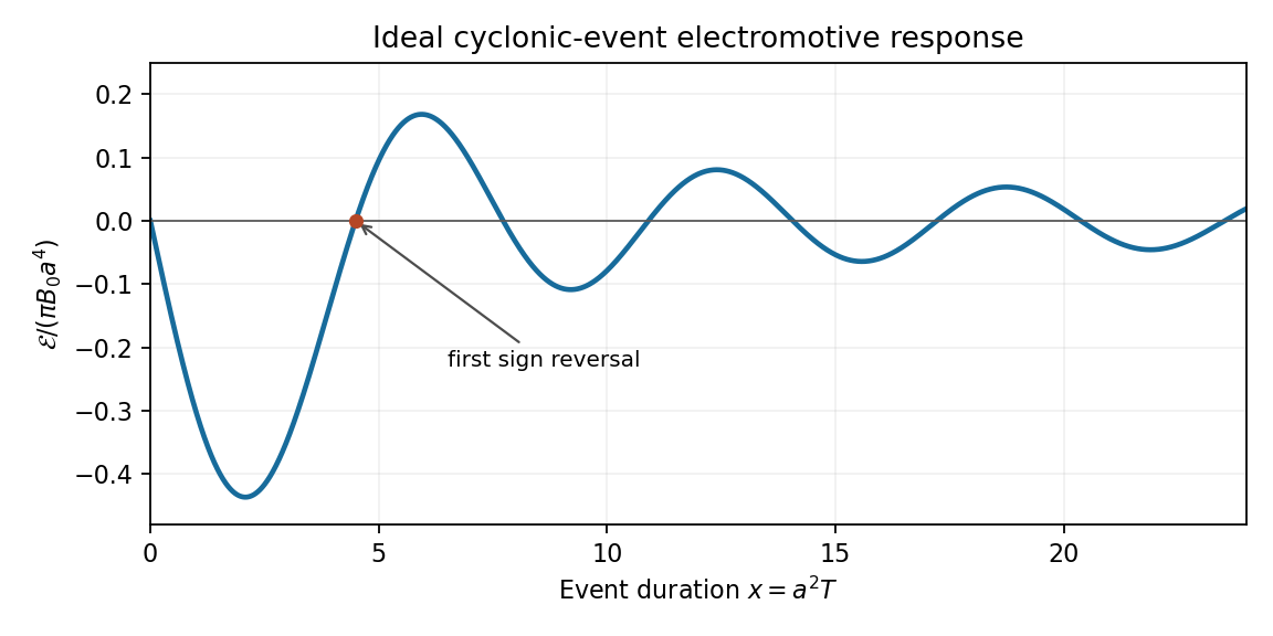
This sign alternation is possible even though the flow has fixed-sign kinetic helicity. Indeed, its vorticity components are $(0,-g^{\prime },2f+r{f}^{\prime })$, so $\mathbf{u}\cdot \mathbf{\omega }=2fg+r(g{f}^{\prime }-f{g}^{\prime })$, which reduces to $2f^2\ge 0$ for this profile. The finite-duration response retains winding and phase information; it cannot be assigned a universal sign from the instantaneous helicity alone.

A small magnetic diffusivity replaces the ideal mode equations byDifferential rotation creates radial phase gradients of order $T{f}^{\prime }$, so the resistive damping rate grows like $\eta T^2{f}^{\prime 2}$. Locally, magnetic phase mixing under differential rotation gives an accumulated damping factor of order $e^{-\eta f^{\prime 2}{T}^3/3}$. Thus the ideal result is a good early-time approximation but diffusion eventually limits winding and stretching, smooths the sharp field gradients at $r=a$, and modifies the later EMF oscillations. Small diffusion does not immediately remove all finite-time sign reversals, and a long-time resistive response requires the diffusive boundary-value problem rather than the ideal formula. After the event, the remaining distorted field relaxes by diffusion toward the imposed uniform background.