Miguel A. Quiñones is a cardiologist credited as chair and first author of the American Society of Echocardiography's 2002 recommendations on quantifying Doppler echocardiography. The primary report's byline gives his name and role, while its technical sections explain how acquisition methods determine the interpretation of recorded velocities.^[ref]

The report distinguishes pulsed-wave Doppler echocardiography, which selects a sampling region but has pulse-rate aliasing limits, from continuous-wave Doppler echocardiography, which records high velocities without unique depth localization. This distinction is central when turning a spectral envelope into a physiological estimate: the measured signal must correspond to the anatomical quantity used in the model.^[ref]

An original sensitivity example illustrates another issue emphasized by the report. Under the simplified pressure-difference model $\Delta p\propto v^2$, a velocity underestimate by $10\%$ changes the calculated result byThe derived pressure difference is underestimated by $19\%$, even before other model errors are considered. For a stipulated estimate of $36\mathrm{mmHg}$ at the true velocity, the underestimated velocity gives $29.16\mathrm{mmHg}$. These numbers illustrate the quadratic mapping rather than provide a clinical threshold or a patient result.

The report explicitly notes this amplification when discussing beam orientation and pressure estimates.^[ref] The contribution documented here is a practical, quantitative measurement framework. Reproducibly tracing a waveform and establishing the accuracy of a derived physiological value remain different tasks.

Pascale Garaud is an applied mathematician and astrophysicist whose work connects fluid dynamics, turbulence and the evolution of stars. Her institutional biography identifies research on stellar flows, magnetohydrodynamics and double-diffusive convection, using both analytical and computational methods.^[ref]

With collaborators, she developed a model for mixing by fingering convection and tested it against three-dimensional direct numerical simulations. A stellar layer can resist ordinary overturning while still mixing because heat and composition diffuse at different rates. Predicting the resulting transport matters when a one-dimensional stellar calculation cannot resolve the individual turbulent motions.^[ref]

Her lecture notes explain how competing thermal and compositional density effects lead to double-diffusive convection. The connection is scientifically useful: a process familiar from salt water becomes relevant to material redistribution inside stars, with very different diffusivity ratios.^[ref]

Portrait: Simons Foundation speaker profile, identified portrait of Pascale Garaud.

A list-decoding algorithm takes a received word $y\in {\Sigma }^n$ and a radius $t$, and outputs every codeword $c$ of a specified block code with Hamming distance $d_H(c,y)\le t$. Correctness requires both completeness and exclusion of more distant words. The running time must also accommodate the output size.

A direct algorithm enumerates all codewords, computes each Hamming distance in $O(n)$ symbol comparisons, and retains the qualifying words. For a binary code with $2^k$ codewords, this costs $O(n{2}^k)$, even if the final list is short. Efficient list decoding exploits algebraic or combinatorial structure instead. For Reed-Solomon codes, polynomial interpolation followed by factorization supplies candidates beyond the unique decoding radius; the candidates are finally checked against the received word.^[ref]

Relocation (computing) adjusts references in program components to match the addresses assigned during linking or loading. A relocation record identifies a place to patch, a target symbol and an architecture-dependent rule for computing the replacement. Moving a section changes the addresses associated with its contents, even when their relative arrangement stays fixed.^[ref]

In an illustrative absolute-address rule, a symbol address $S$ and addend $A$ produce $S+A$. In a relative rule defined using reference address $P$, they may produce $S+A-P$. If $S=4176$, $P=4096$ and $A=0$, the latter gives an offset of $80$. Actual instruction encodings specify the precise reference point, scaling and allowed range, so a linker (computing) must apply the relocation type's rule rather than blindly adding one constant everywhere.

Spectral theory studies a linear operator through the scalars at which it fails to be invertible in the required sense. For a bounded operator $T$ on a complex Banach space, its spectrum consists of $\lambda$ for which $T-\lambda I$ has no bounded inverse defined on the whole space.

In finite dimensions this is the set of eigenvalues. In infinite dimensions there can be more: multiplication by $x$ on $L^2([0,1])$ has spectrum $[0,1]$ but no eigenvectors. An eigenfunction at $\lambda$ would have to be supported on the single point $x=\lambda$, a null set. Functions concentrated near that point nevertheless have arbitrarily small $\Vert (T-\lambda I)f\Vert /\Vert f\Vert$, ruling out a bounded inverse.

Bending changes the curvature of an elastic beam, rod or sheet. In the elementary beam model, material on opposite sides of the neutral axis stretches and shortens. Their longitudinal normal stresses can balance to give zero resultant force while still transmitting a nonzero bending moment. A bent ruler illustrates why resistance to changing shape cannot be described by axial stretching alone.

For a homogeneous slender elastic beam in small-deflection pure bending, take $x$ along the beam and $y$ perpendicular to its centroidal neutral axis. Let $\kappa$ be the signed centreline curvature. The plane-section kinematics and Hooke's law giveHere $E$ is Young's modulus, taken constant over the section. Choosing the positive bending moment as $M=-{\int }_{A}y{\sigma }_{xx}dA$ yieldsThus the second moment of area $I$, rather than just the cross-sectional area, controls bending stress. The beam flexural rigidity is $EI$. Zero axial resultant requires ${\int }_{A}ydA=0$, locating the neutral axis at the section centroid under these assumptions.^[ref]

A four-point bending test makes the constant-moment region experimentally accessible. Two outer supports carry a specimen while two inner contacts apply the load. The Illinois teaching laboratory uses adjustable inner and outer spans on an Instron 4400 frame and records load and deflection electronically; it also tests notched specimens to examine stress concentration.^[ref]

For an original symmetric loading example, place the outer supports at $x=0,L$ and apply total downward force $P$ equally at $x=a,L-a$, with $0<a<L/2$. Each support reaction is $P/2$. Between the inner contacts the transverse shear force is zero and the bending moment is constant, $M=Pa/2$. This central interval realizes the ideal beam conditions for pure bending away from contact disturbances. A three-point bending test instead has its maximum moment at the single central loading contact.

Choose $L=160\mathrm{mm}$, $a=40\mathrm{mm}$, $P=40\mathrm{N}$, rectangular width $b=10\mathrm{mm}$ and thickness $h=4\mathrm{mm}$. Then $I=b{h}^3/12=53.333\mathrm{m}{\mathrm{m}}^4$ and $M=0.800\mathrm{N}\mathrm{m}$. With stipulated $E=70\mathrm{GPa}$, the model givesThese independently chosen numbers describe an assumed elastic specimen, rather than measurements of a particular material.

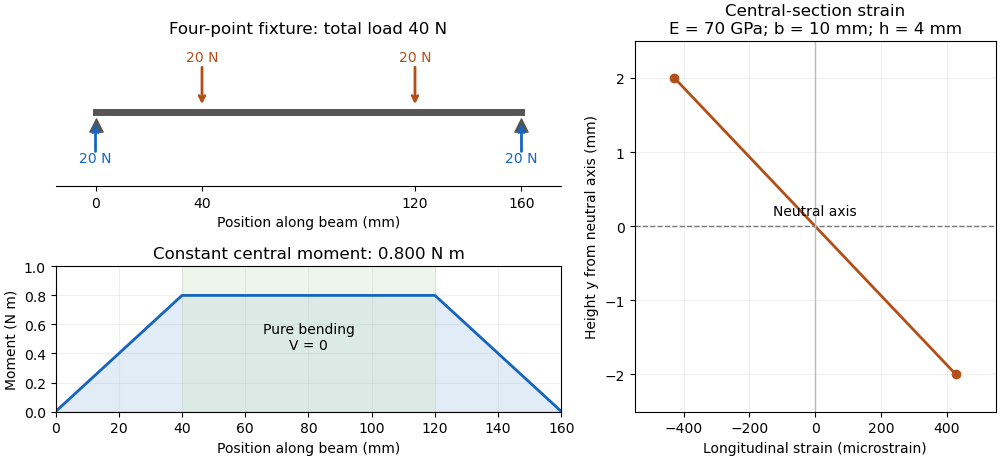
The same relation can infer a flexural modulus from a measured bending moment and curvature, provided the geometry and beam assumptions are adequate. Added axial force contributes a uniform longitudinal normal stress and can shift the zero-stress line. Short beams require attention to transverse shear strain; large rotations require a geometrically nonlinear description. The small-deflection Euler-Bernoulli beam equation and the more general Euler elastica cover different levels of that modeling.

A stress concentration is a localized increase of stress caused by geometry or another disturbance of the load path. Holes, notches and abrupt section changes can make the largest local normal stress much greater than a stress calculated from the total force divided by a reference cross-sectional area. A stress concentration factor $K_t={\sigma }_{\max }/{\sigma }_{\mathrm{ref}}$ is meaningful only after both the stress component and its reference have been specified.

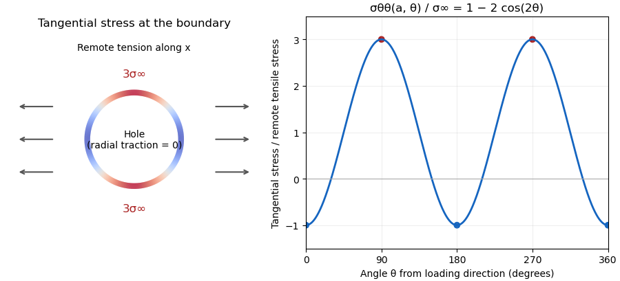
The Kirsch equations give an instructive exact result for a circular hole of radius $a$ in an infinite, isotropic linear elastic elastic plate under remote tensile stress ${\sigma }_{\infty }$ in one direction, using a plane stress model. Measure the polar angle $\theta$ from the loading direction. At the hole boundary,At $\theta =\pi /2,3\pi /2$, the tangential normal stress reaches $3{\sigma }_{\infty }$, giving $K_t=3$ relative to remote stress. At $\theta =0,\pi$, it is $-{\sigma }_{\infty }$. A traction-free hole therefore does not require every component of its stress tensor to vanish: it requires zero traction on the radial boundary.^[ref]

For a finite plate, distinguish gross and net reference areas. A plate of width $W$, thickness $t$ and central hole diameter $d$ transmits force $P$ through gross area $A_g=tW$ and minimum net area $A_n=t(W-d)$. Defining ${\sigma }_g=P/A_g$ and ${\sigma }_n=P/A_n$ gives the exact conversionThis is a change of normalization, not a solution for the finite plate's stress field. For an original numerical example, take $W=40\mathrm{mm}$, $t=2\mathrm{mm}$, $d=10\mathrm{mm}$ and $P=800\mathrm{N}$. The reference stresses are $10$ and $13.333\mathrm{MPa}$. If the local maximum is stipulated as $32\mathrm{MPa}$, the same physical maximum gives $K_{tg}=3.2$ and $K_{tn}=2.4$. Neither number changes the local stress by choosing a different denominator.

The distinction appears in real historical measurements. In 1939, C. Dumont loaded a perforated aluminum-alloy plate in out-of-plane bending and measured strain and deflection at two loads. The reported peak tangential stress was 1.59 times the computed net-section stress, but 1.85 times the computed stress for an unperforated plate under the same bending forces. These are bending results for that geometry, rather than the infinite-plate tensile factor three.^[ref]

Modern demonstrations can combine a metal plate instrumented with strain gauges and a transparent polymer viewed in a polariscope. The latter uses stress-induced birefringence; its fringes respond to differences of principal stresses. The MIT laboratory compares local and remote strain measurements with qualitative photoelasticity observations around holes and a slot.^[ref]

The elastic stress concentration factor is dimensionless. It differs from the stress intensity factor used to describe a sharp crack's singular field. Local yielding or a crack changes the mechanical problem; multiplying a remote stress by the elastic $K_t$ does not, by itself, establish a failure load.

The principle of transmissibility states that moving a force along its line of action preserves its external mechanical effect on an ideal rigid body. The force vector is unchanged, and its torque about every reference point is unchanged. The statement concerns external rigid-body motion or equilibrium; it does not assert unchanged internal deformation.

For an original proof, a nonzero force $\mathbf{F}$ is applied at $\mathbf{r}$. Move it to $\mathbf{r}+s\hat{\mathbf{F}}$, where $\hat{\mathbf{F}}=\mathbf{F}/\Vert \mathbf{F}\Vert$ and $s$ is a signed distance. The new moment isThe last cross product vanishes because its vectors are parallel. This is the same moment geometry used in the primary torque definition.^[ref]

For a numerical example, let $\mathbf{F}=(0,10,0)\mathrm{N}$ act at $(0.30,0.20,0)\mathrm{m}$. Its moment is $(0,0,3)\mathrm{N}\mathrm{m}$. Moving the application point to $(0.30,0.80,0)$ preserves that moment because the displacement follows the force direction. Moving it instead to $(0.50,0.20,0)$ gives $(0,0,5)\mathrm{N}\mathrm{m}$. The second move needs an additional compensating couple to preserve the original wrench.

A one-dimensional elastic counterexample shows the rigid-body limitation. Consider a uniform bar along $0\le x\le L$, fixed at the left end, with a rightward axial force $F$ applied to a cross-section at $x=a$. In a small-strain axial model, internal force is $F$ on $0<x<a$ and zero on $a<x<L$. Its right-end displacement iswhere $E$ is Young's modulus and $A$ the section area. Applying the same force at $a=L$ instead gives $FL/(EA)$, although both applied forces share one line of action and give the same external resultant and moment.

With stipulated $F=100\mathrm{N}$, $L=1\mathrm{m}$, $E=200\mathrm{GPa}$ and $A=1\mathrm{m}{\mathrm{m}}^2$, the end displacement is $0.25\mathrm{mm}$ for $a=L/2$ and $0.50\mathrm{mm}$ for $a=L$. The linear stress–strain relation underlying that calculation is described in the primary elasticity section.^[ref]

A proposed comparison therefore measures support reaction and body deformation separately when changing load position along a common line. Equal reactions and moments can coexist with different local stress and displacement. The external free-body diagram may be equivalent while the internal loading model differs.

A font line gap is a font-wide metric giving an additional spacing allowance to combine with font ascent and font descent. For an elementary default line-spacing calculation using signed descent $d_f$,where $a$ is the ascent and $g$ the font line gap. OpenType's sTypoLineGap is intended to be used with the matching sTypoAscender and sTypoDescender fields.^[ref]

Suppose the chosen metrics are $a=760$, $d_f=-240$ and $g=100$ font units. The default spacing is 1100 font units. With 1000 font units per em at 18 pixels per em, that is 19.8 pixels between text baselines.

The stored font line gap provides an input to a spacing decision. An application can instead request a different line height, and CSS leading is then calculated from that requested height and the selected metrics. Nor does the font line gap measure the visible blank strip between every pair of lines: the ink bounding boxes vary with the particular glyphs. The line height diagram shows this distinction with schematic ink inside larger font-wide metric regions.

Typographic leading concerns vertical spacing between lines of type. The term comes from the thin lead spacers used to separate lines of metal type. In current discussion, one must establish whether a quoted value means the complete spacing between text baselines or an additional allowance beyond the chosen font ascent and font descent.^[ref]

CSS leading uses the additional-allowance convention. If a single font contributes ascent $A$ and descent magnitude $D$, and the chosen line height is $H$, thenThe elementary inline-box construction allocates half of $L$ above the ascent and half below the descent. These quantities are font-wide metrics, rather than the actual ink bounding box of each glyph.^[ref]

For hypothetical metrics $A=11$, $D=3$ and $H=18$ CSS pixels, the extra leading is 4 CSS pixels, with 2 on each side. If the same metrics use $H=12$, then $L=-2$: the allocated line region is smaller than the metric extent. Negative CSS leading is allowed, so visible ink can extend outside its line allocation. A line height value must consequently be interpreted together with the font and the layout convention.

A CSS line box is the rectangular region containing the inline content of one line in a CSS inline formatting context. The browser fits successive inline content into lines, using line breaking when necessary, then uses CSS vertical alignment to determine each line's extent. A CSS inline box supplies one contribution to this enclosing region.^[ref]

For ordinary baseline-aligned text, the CSS leading calculation supplies each contribution's height $a_i$ above and depth $d_i$ below the text baseline. Include the CSS strut among those contributions. Enclosing them requiresFor example, extents $(a_1,d_1)=(10,4)$ and $(a_2,d_2)=(17,3)$ CSS pixels produce a line of $17+4=21$ CSS pixels, although the individual extents sum to 14 and 20. The largest upper extent and largest lower extent can come from different contributions. The CSS leading diagram illustrates the same geometry with another pair of hypothetical metrics.

A CSS replaced element, such as an inline image, contributes according to its CSS margin box; it need not follow the text's line height. Other settings of CSS vertical alignment require additional positioning rules. These effects explain why a line's final height can exceed the line-height declared on its surrounding CSS block container.^[ref]

A bound vortex in an aerodynamic model is a vortex-filament representation attached to the modeled lifting body, rather than a wake element convected downstream. In lifting-line theory, a spanwise distribution of circulation $\Gamma (y)$ represents the wing loading. The word bound describes the representation's relation to the body; it does not identify a literal tube of fluid fixed inside the wing.

The local Kutta–Joukowski theorem connects the modeled circulation to lift per unit span:The MIT derivation uses that connection to couple the section law to the induced flow.^[ref] Here $c(y)$ is airfoil chord; the sign of $\Gamma$ is chosen consistently with positive lift.

An original example stipulates $\rho =1.2$ kg/m${}^3$, $U=40$ m/s and $\Gamma =5$ m${}^2$/s at one section. The predicted $L^{\prime }$ is 240 N/m. For chord 0.50 m, $q=960$ Pa and $c_l=240/(960\cdot 0.50)=0.50$. The same circulation at a different chord need not give the same sectional coefficient.

The finite-span model includes the wake. A horseshoe vortex joins a finite bound segment to trailing legs; continuously varying spanwise circulation generates a distributed trailing vortex sheet. Adjacent modeled segments with circulations 5 and 3 m${}^2$/s have a circulation difference of magnitude 2 m${}^2$/s, which determines the intervening wake-filament strength under the chosen orientation. Omitting those trailing contributions would omit the downwash that couples the wing sections.

Total lift follows from $L=\rho U\int \Gamma (y)dy$, but that single integral does not uniquely determine the distribution. Different span loadings can have equal total lift and different lift-induced drag; the originating force calculation keeps the circulation distribution when evaluating drag.^[ref]

A proposed apparatus comparison reconstructs section loading from surface pressures and independently measures the downstream velocity field. Agreement tests the lifting-line representation and wake prediction. A force reading alone cannot locate a unique physical vortex filament, and the model does not resolve the full viscous flow near the surface.

The induced angle of attack ${\alpha }_i$ is the change between the geometric flow direction and the local effective flow direction caused by the wing's induced velocity. In the usual small-angle lifting-line theory convention, downward downwash is positive andHere $U$ is the reference streamwise speed and $w$ the local downward speed. The originating lecture notes explicitly distinguish geometric, induced and effective incidence.^[ref]

If the local velocity has only these two components, its geometric inclination is $\arctan (w/U)$. The ratio $w/U$ is the small-angle approximation, with angles in radians. An original example uses $U=40$ m/s and $w=1.0$ m/s: ${\alpha }_i=\arctan (0.025)\simeq 1.432{}^{\circ }$. A geometric incidence of $5{}^{\circ }$ then gives effective incidence about $3.568{}^{\circ }$. This does not subtract the zero-lift angle of attack, which is a separate term in the section lift law.

For ideal elliptic span loading, the angle is constant across the span and approximatelyThe latter relation is the lift-induced drag contribution, with unit span efficiency factor.^[ref] For stipulated $C_L=0.60$ and $AR=8$, the approximation gives ${\alpha }_i\simeq 0.02387$ radians and $C_{D_i}\simeq 0.01432$.

A nonuniform wing generally has different local induced angles. Its total induced drag involves the loading-weighted integral $D_i\simeq \int L^{\prime }(y){\alpha }_i(y)dy$; an unweighted arithmetic mean of wake angles need not reproduce that integral. A wake velocity traverse and sectional surface pressure integration for airfoil lift test different pieces of this prediction.

The angle concerns induced flow at the modeled lifting line. A velocity measurement far downstream requires the corresponding wake model before being substituted into this formula. The small-angle, attached-flow approximation also does not account for all sources of drag or for strong crossflow.

The section lift-curve slope $a_0$ is the local derivative of a two-dimensional section lift coefficient with respect to its effective angle of attack, at stated flow conditions:The local linear approximation is $c_l\simeq a_0({\alpha }_{\mathrm{eff}}-{\alpha }_0)$, where ${\alpha }_0$ is the zero-lift angle of attack. Lifting-line theory uses this section relation while separately solving for the induced flow from the finite wing.^[ref]

The angle unit matters. In incompressible thin airfoil theory, the ideal slope is $2\pi$ per radian, or $2\pi (\pi /180)\simeq 0.1097$ per degree.^[ref] A tabulated slope of 0.10 per degree is about 5.73 per radian. Treating 0.10 as a per-radian value introduces a factor of about 57.3.

For an original section model with $a_0=6.0$ per radian and ${\alpha }_0=-2{}^{\circ }$, an effective incidence of $3{}^{\circ }$ givesThe relevant angular increment is five degrees, not three. With sectional dynamic pressure $q=500$ Pa and airfoil chord $c=0.30$ m, the resulting lift per unit span is $L^{\prime }=qc{c}_l\simeq 78.54$ N/m.

The finite-wing lift-curve slope is different because increased lift changes the downwash. For an ideal untwisted elliptic wing with uniform section slope, ${\alpha }_i=C_L/(\pi AR)$ givesTaking $a_0=2\pi$ and wing aspect ratio $AR=8$ yields $a\simeq 5.027$ per radian. This particular reduction is a consequence of the stated ideal loading, not a universal correction for arbitrary swept or separated wings.

A proposed wind tunnel measurement fits nearby section-force measurements against incidence while recording Reynolds number and Mach number. The fitted interval should remain within the approximately linear regime; aerodynamic stall can make one constant slope inadequate.

The maximum lift-to-drag ratio is the largest attainable ratio of positive lift to drag within stated operating conditions. It depends on both the drag polar and the range of lift coefficients the vehicle can actually attain.

For the positive parabolic drag polar $C_D=C_{D0}+k{C}_L^2$, a short proof uses the arithmetic-geometric mean inequality:Consequently
provided that coefficient is attainable. Equality requires equal modeled zero-lift and lift-dependent drag contributions. This bound supplies a global argument, rather than merely locating a stationary point by differentiation.

A lift-constrained maximum lift-to-drag ratio can be lower. With $C_{D0}=0.020$, $k=0.050$ and allowed $0<C_L\le 0.50$, the unconstrained optimum $C_L^{\ast }\simeq 0.6325$ is excluded. Since the ratio increases up to that point, the constrained optimum is at $C_L=0.50$, giving $L/D=15.3846$, below the unconstrained $15.8114$. A stall-limited interval should therefore be applied before claiming the fitted optimum is reachable.

Parameter bounds on maximum lift-to-drag ratio follow from monotonicity. If $C_{D0}\in [c_{-},c_{+}]$ and $k\in [k_{-},k_{+}]$ are positive intervals, then the unconstrained maximum lies in
This interval arithmetic bound is conservative when the fitted parameters are correlated and not all interval combinations are jointly possible. It quantifies uncertainty in the assumed polar; it does not include failure of the polar model itself.