Topics (384k) Articles (398k) Users (410) Discussions (242) Comments (383) Files (13k) New article

D. J. Thompson coauthored the 1952 general treatment of sampling without replacement from a finite population with unequal selection probabilities. The paper with D. G. Horvitz is the source of the Horvitz-Thompson estimator.[ref]
A Generalization of Sampling Without Replacement From a Finite Universe by D. G. Horvitz and D. J. Thompson. Original byline and publisher abstract, pp. 663–685
The contribution separates unbiased total estimation from assumptions of independent selection. If is an inclusion indicator, then , while pair products satisfy . Consequently, for fixed population values,This identity makes joint inclusion probabilities essential to a variance calculation, even though the expectation of the total estimate only needs the individual inclusion probabilities.
For an illustrative population , sample one unit uniformly. Each selected value is multiplied by , so the total estimate is always and its variance is zero. The individual random contributions are nevertheless variable: their covariance cancels their variances because they cannot both be selected. Ignoring that sampling dependence would give the wrong precision. The example shows why design-based estimation concerns the whole selection mechanism, not just a set of multipliers.
Debashis Ghosh is a biostatistician whose research includes recurrent-event methods, statistical machine learning and biomarker evaluation. The Colorado School of Public Health identifies him in its Department of Biostatistics and Informatics. His fuller name is also printed directly in the publisher’s byline for the 2000 paper with D. Y. Lin.[ref]
Debashis Ghosh profile at the Colorado School of Public Health. Institutional directory, research description
[ref]That joint paper studies the mean cumulative number of recurrent events when an event such as death terminates further recurrence. Its contribution is statistical estimation and inference for a stated population quantity, rather than assuming that each observed event is an independent new person.[ref]
Ghosh’s 2010 single-author paper further examines recurrent-event analysis with dependent censoring, linking artificial-censoring methods with truncated-data structures and pairwise estimation. The point is to state and handle a particular observation mechanism, not to claim that every missing-data problem has the same correction.[ref]
An original observation example explains the motivation. If individuals with many events are more likely to stop being followed, an unadjusted mean of observed counts can look low because later events are hidden. If a terminal event is actually observed, later events are precluded instead. Recording why observation ends is therefore part of interpreting the data, alongside the count itself. These distinctions connect Ghosh’s documented work to survival analysis, counting processes and reproducible statistical definitions.
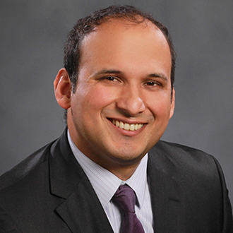
Debashis Ghosh
. Portrait linked from the named Colorado School of Public Health directory profile.D. Y. Lin coauthored the 2000 primary paper on nonparametric analysis of recurrent events and death with Debashis Ghosh. Its target is the marginal mean cumulative count of events in the presence of a terminal event, with estimation, covariance-based inference, simulation assessment and an application to a cancer trial. The publisher identifies Lin as the corresponding author.[ref]
Nonparametric analysis of recurrent events and death by D. Ghosh and D. Y. Lin. Publisher byline and abstract; Biometrics 56(2), 554–562
The statistical problem is that death ends the possibility of later events while preserving the events that occurred earlier. Let count qualifying events up to time , stopping at death. The population mean differs from an average calculated only among those alive at .
An original two-person illustration makes the distinction explicit. In one complete history, an individual dies after zero events and the surviving individual has one; mean accumulated count per original individual is . In another history, the deceased individual had four events before death while the survivor again has one; the mean is . The survivor-only mean is one in both histories. Knowledge of the surviving group alone therefore cannot recover the original cohort’s accumulated burden.
A count at fixed time is a nonnegative random variable, but estimating its mean with incomplete observation is not merely an arithmetic exercise. Loss to follow-up hides later outcomes; an observed terminal event ends the defined process. Treating both identically can change the quantity being estimated. This is the connection between Lin’s documented recurrent-event work, survival analysis and the careful definition of a statistical endpoint.
Fred C. Leone coauthored the 1961 paper The Folded Normal Distribution by F. C. Leone and others with L. S. Nelson and R. B. Nottingham. The original paper lists Leone at the Case Institute of Technology. Its motivating problem was industrial measurement in which a difference or deviation is retained but its algebraic sign is lost or disregarded.[ref]
The Folded Normal Distribution by F. C. Leone and others. First page, byline/affiliation, abstract and introduction
The resulting folded normal distribution combines two possible signed observations at each positive magnitude. If has normal distribution density and , thenThe negative side is reflected onto the positive side. It is not simply deleted. At zero signed mean this gives the half-normal distribution; a nonzero offset changes the shape while the observation remains nonnegative.
For a concrete constructed example, suppose a measuring device displays distance from a target rather than signed displacement. A true mean displacement and its mirror , at the same standard deviation, give identical recorded-distance distributions. The joint paper treats the distribution and estimation problem induced by that recording convention. Its tables and example connect the mathematical transformation to analysis of measurements.[ref]
The Folded Normal Distribution by F. C. Leone and others. Abstract, moment-based parameter estimation and example
The work illustrates a broader principle of statistical modelling: specify what the instrument records before selecting the data distribution. A measurement transformation can alter the observed shape without any change in the underlying physical variability.

Fred C. Leone
. Portrait linked in Purdue University's 1993 Distinguished Alumnus Fred C. Leone by Purdue University notice.L. S. Nelson is a coauthor, with F. C. Leone and R. B. Nottingham, of the 1961 paper The Folded Normal Distribution by F. C. Leone and others. It develops estimation of the underlying normal distribution's mean and standard deviation from measurements reported as absolute values, with tables and an example to support the procedure.[ref]
The Folded Normal Distribution by F. C. Leone and others. Publisher abstract, estimation problem and tabulated assistance
The distinction between the observed mean and the signed mean is important. For with , , soA second moment alone does not separate offset from spread. For example, and both give , although their full folded normal distributions differ. Additional distributional information or moments are needed to distinguish these cases.
When , the observed mean is , about , rather than zero. Interpreting the average absolute deviation as the original signed mean would therefore create an apparent positive offset even for a centered normal distribution. These elementary consequences explain the measurement problem addressed by the joint paper; they are illustrative derivations rather than an attribution of a particular calculation to Nelson alone.
R. B. Nottingham coauthored The Folded Normal Distribution by F. C. Leone and others with F. C. Leone and L. S. Nelson, published in Technometrics in 1961. Their paper addressed measurements whose algebraic signs were not recorded. Even if a signed quantity follows a normal distribution, its recorded magnitude follows a different probability distribution.[ref]
The Folded Normal Distribution by F. C. Leone and others. Primary byline, abstract and introduction: unsigned measurements and parameter estimation
The practical issue is information loss during observation. If and the instrument reports , then and produce the same folded normal distribution. Thus magnitudes alone cannot distinguish an offset to one side of a reference from an equally large offset to the other side. This conclusion follows from the observation rule, not from the quality of a numerical fitting method.
An illustrative inspection records distances from a reference line but omits which side each point lies on. A pair of signed readings and becomes two identical magnitudes . Retaining the original signs would preserve a distinction that no later analysis of those two magnitudes can reconstruct. The paper's contribution is to treat this altered observation distribution explicitly rather than fit an ordinary signed normal distribution to magnitude data.
The cited work is jointly authored; the primary byline does not assign individual responsibility for particular formulas or tables. The printed initials are retained here without attaching unrelated biographical records to this author.
Thomas J. Rothenberg is a mathematical econometrician whose work concerns statistical inference and the identifiability of models. The American Economic Association's 2015 citation recognizes his contributions to identification and inference and identifies him as a professor emeritus at Berkeley.[ref]
Thomas Rothenberg, Distinguished Fellow 2015 by the American Economic Association. Award citation and institutional identification
His primary paper Identification in Parametric Models by Thomas J. Rothenberg, published in 1971, develops identification criteria beyond one model considered in isolation. It connects local identification with the information matrix under regularity conditions and treats identification of individual parameters separately from that of the full vector.[ref] The distinction is useful when a scientifically relevant combination is recoverable even though the entire parameterization is not; identifiability from linear observations gives an explicit example.
An original counterexample explains why the regularity qualifications matter. Consider one observation with normal distributionThe mean map is one-to-one, so distinct parameters have distinct observable distributions. Nevertheless its Fisher information iswhich vanishes at zero. The information rank changes there, so a nonsingularity criterion cannot be applied without its assumptions. Nonregular identification at a flat mean map separates exact distinguishability from first-order sensitivity: a zero derivative does not by itself establish that two different parameter values produce the same law.
The example illustrates a broader contribution of identification theory. Before asking an estimator for a precise answer, determine whether the observations can distinguish the proposed quantities and whether the local approximation used for inference is valid.

D. R. Enzmann is the radiologist credited under that byline as first author of Normal flow patterns of intracranial and spinal cerebrospinal fluid defined with phase-contrast cine MR imaging by D. R. Enzmann and others. With N. J. Pelc, Enzmann reported measurements of moving cerebrospinal fluid, using magnetic resonance imaging to investigate physiology as well as anatomical appearance.[ref]
Normal flow patterns of intracranial and spinal cerebrospinal fluid defined with phase-contrast cine MR imaging by D. R. Enzmann and others. Radiology 178 (1991), 467–474; verified byline and abstract.
The study examined ten healthy volunteers and four patients whose conventional MR images were normal. Peripheral gating produced sixteen quantitative flow-encoded images over the cardiac cycle. Measurements distinguished the timing of fluid motion in ventricular and subarachnoid spaces, demonstrating why static anatomy alone does not describe pulsatile movement.[ref]
Normal flow patterns of intracranial and spinal cerebrospinal fluid defined with phase-contrast cine MR imaging by D. R. Enzmann and others. Abstract: participant groups, peripheral gating and regional flow timing.
The methodological contribution is an example of turning image contrast into a physiological measurement. Direction-sensitive signals and repeated sampling across a heartbeat distinguish oscillatory motion from a compartment that simply looks fluid-filled. The reported display convention assigned opposite intensities to opposite craniocaudal directions; that convention belongs to the acquisition and is not a universal rule for brightness in every MR image.
N. J. Pelc is a coauthor with D. R. Enzmann of a 1991 study that used phase-contrast magnetic resonance imaging to measure cerebrospinal fluid motion through the cardiac cycle. The work illustrates how magnetic resonance imaging can provide a time-dependent physiological measurement rather than only an anatomical picture.[ref]
Normal flow patterns of intracranial and spinal cerebrospinal fluid defined with phase-contrast cine MR imaging by D. R. Enzmann and others. Radiology178,467–474(1991), originating byline and abstract.
The investigators studied ten healthy volunteers and four patients whose conventional magnetic-resonance images were normal. Peripheral cardiac gating divided the measurement into 16 flow-encoded images per cycle. The flow encoding distinguished opposite directions of cerebrospinal fluid motion, and measurements at several locations showed that the timing of the motion differed between the ventricular system and surrounding spaces.[ref]
Normal flow patterns of intracranial and spinal cerebrospinal fluid defined with phase-contrast cine MR imaging by D. R. Enzmann and others. Abstract: participant groups,16 cardiac phases, directional encoding and regional timing.
For an illustrative one-second cycle, 16 equally spaced phases would separate samples by seconds. The paper's number of cardiac phases therefore matters: an average over the entire cycle could hide changes of direction within it. Conversely, sixteen phases are a temporal sampling scheme, not evidence of sixteen independent subjects. This example explains the measurement design without assigning an unreported individual contribution to either coauthor.
Charles T. Dotter was a radiologist whose work helped establish interventional radiology: using imaging-guided vascular access to treat disease as well as visualize it. His Oregon institution credits his 1964 percutaneous transluminal angioplasty with launching that approach. With Melvin P. Judkins, he reported the development of catheter-based treatment for arterial obstruction.[ref]
https://www.ohsu.edu/dotter-interventional-institute. OHSU, Dotter's legacy of innovation:1964 image-guided transluminal angioplasty
[ref]Percutaneous Transluminal Treatment of Arteriosclerotic Obstruction by Charles T. Dotter and Melvin P. Judkins. Radiology 84(1965),631–643, originating byline and abstract.
The motivating observation was mechanical as well as radiological. Their 1965 report discussed catheter pathways through or alongside obstructed arterial material and illustrated contrast visualization of such passages. An event that could complicate diagnostic catheterization suggested that a new flow path might also be deliberately useful. The report framed the approach as a treatment for obstruction, rather than merely a way to obtain a sharper radiograph.[ref]
Percutaneous Transluminal Treatment of Arteriosclerotic Obstruction by Charles T. Dotter and Melvin P. Judkins. Developmental Background and Figures 1–2; stated therapeutic purpose.
A separate idealized flow calculation explains why lumen size matters. For a long circular tube carrying steady laminar flow of a Newtonian fluid, with fixed pressure difference, length and viscosity, flow is proportional to the fourth power of the radius. Increasing the radius by a factor of two would increase this model's flow by . Real blood vessels are compliant, flow can be pulsatile and lesions have complicated shapes; the calculation is an explanatory limit, not an outcome predicted for a particular patient.
Dotter's contribution illustrates a scientific change of question: imaging can measure where a passage is obstructed, while an instrument introduced under imaging guidance can alter that passage. Demonstrating instrument passage, restoring flow and establishing durable clinical benefit are distinct evidential steps. The historical report motivates this sequence without making them equivalent.
Melvin P. Judkins was a radiologist who developed preshaped catheters and a percutaneous transfemoral method for selective coronary angiography. His work connected catheter geometry, vascular anatomy and X-ray recording: the instrument had to reach a particular arterial opening, while the imaging system had to record the contrast-filled vessels.[ref]
https://www.scai.org/melvin-p-judkins-md-1922-85. SCAI professional-society account: preshaped Judkins catheters and selective coronary technique
His 1967 report Selective Coronary Arteriography: Part I: A Percutaneous Transfemoral Technic by Melvin P. Judkins described 100 consecutive patients examined for suspected coronary disease. Both coronary arteries were selectively catheterized from femoral access, and contrast injections were recorded by direct serial radiography and cine imaging. The methods describe forming catheter shapes over preformed bending wires, showing that the instrument's geometry was an engineered part of the measurement rather than an incidental tube.[ref]
Selective Coronary Arteriography: Part I: A Percutaneous Transfemoral Technic by Melvin P. Judkins. Abstract, Material and Technic, including original catheter-shaping description.
For an illustrative contrast experiment, imagine comparing a broad injection upstream with a small injection at the opening of one branch. The latter changes where contrast first enters and can make the selected branch easier to distinguish. That qualitative comparison explains the word selective; it does not specify a safe injection protocol or claim equal performance in every anatomical arrangement.
Judkins also collaborated with Charles T. Dotter on transluminal treatment of arterial obstruction, linking diagnostic access to the possibility of treatment through a catheter.[ref]
Percutaneous Transluminal Treatment of Arteriosclerotic Obstruction by Charles T. Dotter and Melvin P. Judkins. Originating 1965 byline, abstract and developmental discussion.
His preshaped coronary instruments and the joint obstruction work are related contributions, but they address different immediate tasks: delineating a vessel and changing an obstructed passage.Peter M. Aronow develops statistical methods for causal inference, particularly design-based inference. Yale's institutional biography identifies research on complex experimental designs, network settings and incomplete survey data alongside appointments spanning political science and statistics.[ref]
Peter M. Aronow profile by Yale School of Public Health. Titles and Biography, design-based methodological research
His joint work with Cyrus Samii studies how to estimate sampling variance when a sampling design never observes some pairs together. A missing product cannot simply be deleted from the population variance formula: doing so can produce either sign of bias. Their construction uses Young inequality to bound unobserved products by individually estimable powers and obtain a conservative variance estimator.[ref]
Conservative variance estimation for sampling designs with zero pairwise inclusion probabilities by Peter M. Aronow and Cyrus Samii. Section2.2, Proposition1; Section3.1, Proposition2; Section3.2, quadratic special case
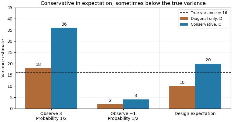
For an original exact illustration, choose one of two fixed values with equal probabilities. As in the single-draw variance identifiability obstruction, the Horvitz-Thompson estimator has true variance . Retaining only diagonal contributions gives , withOpposite signs therefore produce downward bias. The elementary inequality , obtained from , instead givesConsequently is a conservative variance estimator for this stipulated sampling design; its excess in expected value is exactly .
With , the true variance is16. The two possible values of are18 and2, averaging10; those of are36 and4, averaging20. Although , a realized value of can be below16. Conservativeness here is an expectation inequality, rather than a bound for every sample. By itself it also does not prove a specified confidence interval coverage probability.
Cyrus Samii is a political scientist at New York University whose methodological work concerns quantitative field research and causal inference. His academic biography connects the design of randomized controlled trials to empirical social research.[ref]
Affiliations and Bio by Cyrus Samii. Affiliations and Bio, methodology and field-research description

Cyrus Samii
. Portrait linked as cds_self from Samii's personal academic biography; served directly by the original website.With Peter M. Aronow, Samii studied sampling designs in which every unit can be observed but some pairs can never be observed together. The distinction matters: positive individual inclusion probabilities suffice for an unbiased estimator of a finite population total, whereas the usual Horvitz-Thompson variance estimator also needs pairwise inclusion positivity.[ref]
Conservative variance estimation for sampling designs with zero pairwise inclusion probabilities by Peter M. Aronow and Cyrus Samii. Section2, conditions1–2 and Sections2.1–2.2, observable and unobservable cross-products
An original two-unit example makes the single-draw variance identifiability obstruction explicit. Fix two unknown population values and choose one index with probabilities . The Horvitz-Thompson estimator is , soAn estimator based only on the selected index and its observed value has expected value of the form . Such an additive expression cannot equal for every pair of real values. Taking the mixed finite difference at gives zero for the additive expression butfor the desired variance. Thus a single draw permits an unbiased estimator of the total but no universally unbiased estimator of its sampling variance. Independent auxiliary randomization cannot repair this: averaging that randomness still gives functions and of the same observed data.
This is a restriction imposed by the observation mechanism, rather than a shortage of algebraic ingenuity. It motivates separating design-based inference about a total from the additional information needed to quantify its uncertainty.
Paul Boersma is a phonetician who co-created Praat with David Weenink. His work connects acoustic measurements to computational methods, including the estimation of fundamental frequency from sampled speech.[ref]
Praat: doing phonetics by computer by Paul Boersma and David Weenink. Intro, authorship
His 1993 periodicity-analysis paper examines how signal sampling and a finite analysis window affect estimates based on autocorrelation. Repetition produces peaks at nonzero time lags; locating a suitable peak gives a candidate period, while the relative peak height contains information about periodicity. Correcting the influence of the analysis window is important before interpreting those peaks as properties of the original signal.[ref]
Accurate short-term analysis of the fundamental frequency and the harmonics-to-noise ratio of a sampled sound by Paul Boersma. Sections1–3: autocorrelation, windowing and pitch-period estimation
Homepage: www.fon.hum.uva.nl/paul/

David Weenink co-created Praat with Paul Boersma, providing tools for measuring and modeling speech. His 2006 thesis investigated speaker-adaptive vowel identification: how recognition can remain useful when acoustic patterns vary between speakers.[ref]
Praat: doing phonetics by computer by Paul Boersma and David Weenink. Intro, authorship
[ref]The thesis describes recordings from 30 speakers, each producing 12 Dutch vowels in controlled sentence frames. It relates these data to formants, principal component analysis, discriminant analysis and adaptive classification methods. This makes the recognition problem experimentally concrete: a classifier must separate vowel identity from speaker-related variation rather than memorize a single speaker's frequency spectrum.[ref]
Speaker-adaptive vowel identification by David Weenink. Chapters1–3 and11;30-speaker/12-vowel data description
Homepage: www.fon.hum.uva.nl/david/

Gunnar Fant developed acoustic models connecting the physical production of speech to its measurable signal. His Acoustic Theory of Speech Production by Gunnar Fant relates vocal-tract geometry to acoustic behavior, including calculations based on X-ray studies of articulations. The original book dates to 1960; the inspected publisher preview is its 1970 second printing.[ref]
His source-filter model of speech production separates excitation from the filtering of the vocal tract. Changing a filter's resonances can move formants without requiring the same change in the fundamental frequency of the source. This makes speech synthesis an experimental tool: a researcher can vary model parameters and compare the generated signal with recorded speech. KTH's account explicitly describes his synthesis work as a means of testing production hypotheses.[ref]
Human Speech and Communication at KTH. research history, Fant and the experimental role of synthesis
KTH's curriculum vitae records 1919–2009 and his leadership of the Speech Transmission Laboratory from 1951 to 1966.[ref]

https://commons.wikimedia.org/wiki/File:Gunnar_Fant.jpg. Wikimedia Commons file record, named subject and institutional credit
Licensed CC BY-SA 3.0.John Collier is a laser physicist associated with the Central Laser Facility. His Learned Society of Wales profile identifies laser physics as his specialist subject and gives the Rutherford Appleton Laboratory affiliation.[ref]
John Collier profile at the Learned Society of Wales. Fellow profile
The facility's historical account identifies Collier and I. Ross with the development of optical parametric chirped pulse amplification, including a1999 test system. In this technique a pump transfers energy through a nonlinear optical interaction to an already chirped signal; subsequent compression aims to recover a short, high-power pulse.[ref]
CLF: 40 Years in Pictures. Printedp16, Optical Parametric Chirped Pulse Amplification and photograph99RC1329
Collier also coauthored the1999 report on a single-shot diagnostic for third-order intensity autocorrelation.[ref]
A Single Shot 3rd Order Cross-Correlator for Pulse Contrast and Pulse Shape Measurements by J. Collier and others. Printedp194, byline
Amplification and characterization are complementary tasks: increasing the pulse energy does not by itself establish the temporal shape or the quality of compression.For an original comparison, consider two hypothetical pulses with equal energy but rectangular durations of1 and10picoseconds. Their powers differ by a factor10. A measurement of the energy alone cannot distinguish them, while a time-sensitive diagnostic can constrain the missing duration and shape information. More generally, both amplification performance and the delivered temporal waveform matter in interpreting a high-power laser experiment.
Cristina Hernandez-Gomez develops high-power laser technology and experimental facilities. Her Central Laser Facility biography describes work on the Vulcan Petawatt upgrade after joining in1997, followed by leadership of Vulcan and the High Power Lasers Division.[ref]
She coauthored the1999 single-shot pulse-correlation report with the other Central Laser Facility researchers listed in its byline.[ref]
A Single Shot 3rd Order Cross-Correlator for Pulse Contrast and Pulse Shape Measurements by J. Collier and others. Printedp194, byline
The diagnostic problem includes distinguishing a weak, extended signal from the main short pulse.An original rectangular-waveform example separates peak contrast from energy contrast. Let the main pulse have power for1picosecond and a preceding feature have power for100picoseconds. Their energy ratio isThe preceding feature is at0.01% of the main peak, yet contains1% of the main pulse energy in this stipulated model. Reporting only its height would conceal its much longer duration.
This is why optical pulse temporal contrast and laser pulse energy need temporal definitions and a measured waveform. Facility development involves controlling the delivered pulse as well as its nominal peak: the diagnostic should establish what reaches the experiment, over the time interval relevant to that experiment.
Ian N. Ross is a laser researcher identified in Central Laser Facility publications. The1998/99 facility directory gives Ian Ross with the address
[email protected]; a2003 amplifier paper supplies the full byline Ian N. Ross and the same institutional address.[ref]High-performance diode-pumped Nd:YLF amplifier by Ian N. Ross and others. Author information; corresponding address
With Marta Csatári and Steve Hutchins, Ross reported a multipass optical amplifier combining high gain and stable output. The abstract gives saturated gain above6000 and output stability of0.2% rms over the shorter measurement interval and0.7% rms over the longer one under the reported conditions.[ref]
An original interpretation example distinguishes stability from absolute accuracy. If a readout has mean100units and relative standard deviation0.2%, its standard deviation is0.2units. A constant calibration error could shift every reading together while leaving that relative fluctuation small. A stability figure consequently does not by itself establish the correctness of the absolute output scale.
Ross also worked with John Collier on optical parametric chirped pulse amplification, as documented in the facility's historical account.[ref]
CLF: 40 Years in Pictures. Printedp16, OPCPA development and1999 test-system caption
These contributions connect amplifier design with the need to control and characterize the pulses it produces. Gain, stability, spectrum and temporal shape describe different aspects of performance.Ric Allott has worked on photonics research and its industrial applications at the Central Laser Facility. The facility's2017 announcement of his visiting professorship describes a career spanning research, industrial work and technology transfer; it records his first CLF appointment in1995.[ref]
Ric Allott professorship announcement at the Central Laser Facility. Professional background and industrial photonics contributions
Allott coauthored the1999 single-shot optical pulse-correlation report.[ref]
A Single Shot 3rd Order Cross-Correlator for Pulse Contrast and Pulse Shape Measurements by J. Collier and others. Printedp194, byline
Such diagnostic work connects a physical response with a quantitatively interpretable measurement of optical pulse temporal contrast.An original readout example illustrates why that interpretation matters. Normalize a reference peak to1. Suppose a weak feature gives0.0012 in the same units, including a separately measured additive baseline of0.0002. The corrected feature level isOmitting the baseline would overestimate this level by20%. The arithmetic is simple, but its physical validity depends on the baseline being representative and both measurements using a compatible scale.
Moving a diagnostic from a laboratory demonstration into applications therefore involves measurement calibration, reproducibility and a clear account of what its output represents. A large displayed ratio alone does not establish the measurement's accuracy. This example explains one aspect of the scientific-to-application connection without assigning unreported individual experimental tasks to Allott.
Pinned article: Introduction to the OurBigBook Project
Welcome to the OurBigBook Project! Our goal is to create the perfect publishing platform for STEM subjects, and get university-level students to write the best free STEM tutorials ever.
Everyone is welcome to create an account and play with the site: ourbigbook.com/go/register. We belive that students themselves can write amazing tutorials, but teachers are welcome too. You can write about anything you want, it doesn't have to be STEM or even educational. Silly test content is very welcome and you won't be penalized in any way. Just keep it legal!
Intro to OurBigBook
. Source. We have two killer features:
- topics: topics group articles by different users with the same title, e.g. here is the topic for the "Fundamental Theorem of Calculus" ourbigbook.com/go/topic/fundamental-theorem-of-calculusArticles of different users are sorted by upvote within each article page. This feature is a bit like:
- a Wikipedia where each user can have their own version of each article
- a Q&A website like Stack Overflow, where multiple people can give their views on a given topic, and the best ones are sorted by upvote. Except you don't need to wait for someone to ask first, and any topic goes, no matter how narrow or broad
This feature makes it possible for readers to find better explanations of any topic created by other writers. And it allows writers to create an explanation in a place that readers might actually find it.
Figure 1. Screenshot of the "Derivative" topic page. View it live at: ourbigbook.com/go/topic/derivativeVideo 2. OurBigBook Web topics demo. Source. - local editing: you can store all your personal knowledge base content locally in a plaintext markup format that can be edited locally and published either:This way you can be sure that even if OurBigBook.com were to go down one day (which we have no plans to do as it is quite cheap to host!), your content will still be perfectly readable as a static site.
- to OurBigBook.com to get awesome multi-user features like topics and likes
- as HTML files to a static website, which you can host yourself for free on many external providers like GitHub Pages, and remain in full control

Figure 2. You can publish local OurBigBook lightweight markup files to either OurBigBook.com or as a static website.
Figure 3. Visual Studio Code extension installation.
Figure 5. . You can also edit articles on the Web editor without installing anything locally. Video 3. Edit locally and publish demo. Source. This shows editing OurBigBook Markup and publishing it using the Visual Studio Code extension. 
- Infinitely deep tables of contents:




All our software is open source and hosted at: github.com/ourbigbook/ourbigbook
Further documentation can be found at: docs.ourbigbook.com
Feel free to reach our to us for any help or suggestions: docs.ourbigbook.com/#contact