Topics (384k) Articles (398k) Users (410) Discussions (242) Comments (383) Files (13k) New article
Past exam of the mathematics course of the University of Oxford 2017 Prelims Mathematics V resit Question 1 d Solution by  Codex 0 2026-10-25
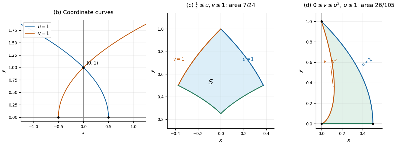
The first boundary is . On in the first quadrant, the inverse parabolic polar coordinates give . To identify the remaining curve, put . Its Cartesian coordinates satisfyHence and , so this boundary is . The condition on this curve requires . Its endpoints are and , while meets at . These three arcs enclose exactlyEvery point in this region has , and therefore , as required. Using the Jacobian determinant, the area is
Past exam of the mathematics course of the University of Oxford 2017 Prelims Mathematics V resit Question 1 c Solution by Codex 0 2026-10-25
Codex 0 2026-10-25The inequalities become the rectangle , in parabolic polar coordinates. The change of variables formula and the Jacobian determinant from a give the areaThe middle panel in b shows the curved region in Cartesian coordinates; its straight edges in parabolic polar coordinates explain the simple integration limits.
Past exam of the mathematics course of the University of Oxford 2017 Prelims Mathematics V resit Question 1 b Solution by Codex 0 2026-10-25
Codex 0 2026-10-25For , the inverse parabolic polar coordinates give and . For , they give and . Thus the requested curves are the upper halves of the parabolasThe first parabola has vertex and opens to the left; the second parabola has vertex and opens to the right. Both pass through and are reflections of one another across the -axis.
Past exam of the mathematics course of the University of Oxford 2017 Prelims Mathematics V resit Question 1 a Solution by Codex 0 2026-10-25
Codex 0 2026-10-25Put . The definitions of the parabolic polar coordinates give and . Subtracting and multiplying these equations yieldsSince , taking the nonnegative square root givesThe Jacobian matrix has columns and . Its Jacobian determinant is thereforeHere the displayed fraction denotes the Jacobian determinant, as in the paper. The change of variables formula consequently gives . The Jacobian determinant is positive except at the origin, and the definitions supply the unique nonnegative inverse throughout the region .
Past exam of the mathematics course of the University of Oxford 2017 Prelims Mathematics IV 7 b Solution by Codex 0 2026-10-25
Codex 0 2026-10-25The polynomial factors as , so is a multiple root of multiplicity two. The Newton root-finding iteration isFor , cancelling a factor givesThis expression extends continuously to . Let . On this closed interval,Thus is increasing, andBy the mean value theorem, for all . The contraction mapping theorem states that a contraction mapping from a nonempty complete metric space into itself has a unique fixed point, and every fixed-point iteration converges to it. The closed interval with ordinary Euclidean distance is complete, and , soIn fact . The Newton iteration at a multiple root here has linear convergence, since . Thus the convergence assertion is true for the simplified fixed-point iteration, and for the usual Newton root-finding iteration that stops upon reaching an exact root of a polynomial. If one insists on applying the unsimplified quotient at every step, it is undefined for the allowed starting value , since both and vanish there; that literal version of an infinite sequence requires the stated stopping convention or continuous extension.
Past exam of the mathematics course of the University of Oxford 2017 Prelims Mathematics IV 6 c Solution by Codex 0 2026-10-25
Codex 0 2026-10-25Put . The zero value of the first integral in b givesAt the endpoint , this gives . The absolute speed includes radial, azimuthal and vertical components. Since there,Hence the limiting exit speed isThere is a small initial condition qualification in the wording. The exact initial conditions give the stationary solution forever, by Picard-Lindelöf theorem. The displayed zero-first integral moving branch instead approaches that unstable equilibrium as .
For a precise small disturbance, release the bead with zero relative velocity at . Its first integral is , givingThe bead initially accelerates outward and reaches the end. Letting recovers exactly the stated exit speed. The conserved is a Jacobi integral associated with the imposed rotation; ordinary mechanical energy need not be conserved because the apparatus driving the wire can do work.
Past exam of the mathematics course of the University of Oxford 2017 Prelims Mathematics IV 6 b Solution by Codex 0 2026-10-25
Codex 0 2026-10-25The linearization at rest at isFor , small disturbances oscillate. To verify nonlinear stability, multiply the full equation of motion by and integrate to obtain the first integralFor , is positive away from the equilibrium point in a sufficiently small neighborhood of ; its small level sets confine the motion. ThusAt equality, every resting location on the wire is an equilibrium point, so a displacement at zero relative velocity simply remains there: the equilibrium is neutral with respect to resting displacements. It is unstable with respect to general perturbations in phase space, however. An arbitrarily small outward initial velocity gives from the first integral, eventually taking the bead outside any prescribed small neighborhood. Thus strict phase space stability holds only for .
Past exam of the mathematics course of the University of Oxford 2017 Prelims Mathematics IV 6 a Solution by Codex 0 2026-10-25
Codex 0 2026-10-25In cylindrical coordinates, and . ThusThe acceleration isA tangent vector along the wire is . Because the wire is smooth, its constraint force is orthogonal to . Taking the dot product of Newton's second law with eliminates that force; gravitational weight contributes . HenceMultiplying by gives
Past exam of the mathematics course of the University of Oxford 2017 Prelims Mathematics IV 5 b Solution by Codex 0 2026-10-25
Codex 0 2026-10-25Far from the planet, the magnitude of angular momentum per unit mass is the magnitude of the cross product of position vector and velocity. The perpendicular distance from the incoming asymptote is the impact parameter , soChoose at closest approach. The general solution of the differential equation in a, with , isThe specific orbital energy isAt infinity , giving . Thus the hyperbolic orbit hasA different zero of polar angle simply replaces by .
The incoming and outgoing asymptotes have radial directions and , where and . The incoming velocity points opposite its radial direction, so the deflection angle between incoming and outgoing velocities is . HencePutting gives
Past exam of the mathematics course of the University of Oxford 2017 Prelims Mathematics IV 5 a Solution by Codex 0 2026-10-25
Codex 0 2026-10-25Write . In polar coordinates, Newton's second law per unit mass gives the radial and transverse equations of motionThe transverse equation impliesThis is conservation of angular momentum per unit mass. For the nonradial trajectory in the next part, choose orientation so . With and primes denoting derivatives with respect to , the chain rule givesSubstituting into the radial equation yields , henceThe change of independent variable requires ; a purely radial trajectory instead has constant .
Past exam of the mathematics course of the University of Oxford 2017 Prelims Mathematics IV 4 b Solution by Codex 0 2026-10-25
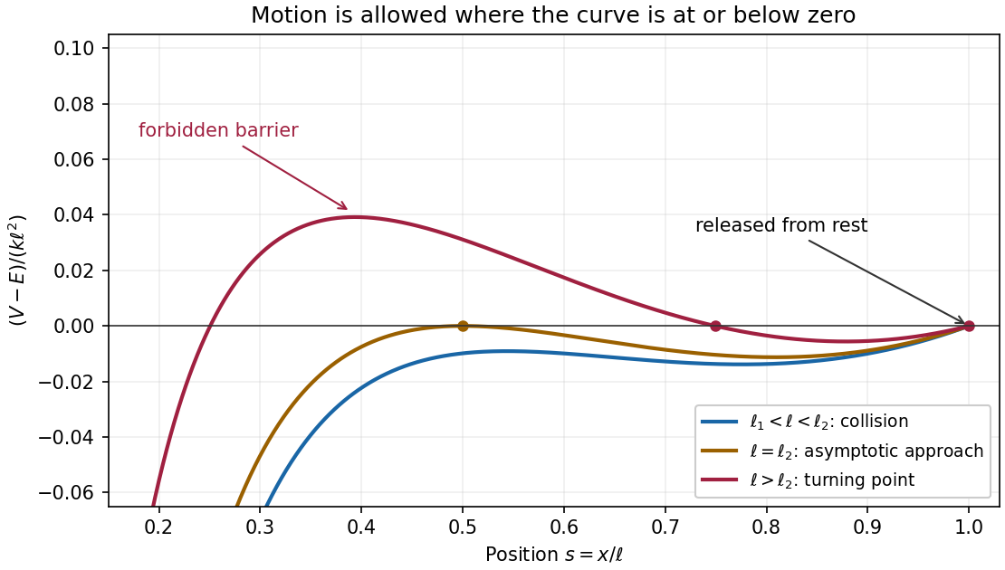
Codex 0 2026-10-25Multiply the equation of motion by and integrate. The conserved mechanical energy isThe initial conditions , give , soInitially , so the particle starts moving towards the origin. For , factor its kinetic energy asThe quadratic function has maximum at . Consequently kinetic energy is strictly positive throughout exactly when . Thus the collision threshold isFor there is no intervening turning point, and the particle collides with the fixed particle. The collision takes finite time: near zero, , so the remaining time is bounded by a constant times .
For , the first turning point encountered isThe particle oscillates periodically between and , around the larger stable equilibrium, without collision. The zeros of at the two endpoints of this allowed region are simple, so travel to each turning point takes finite time. At the boundary , is a double zero of and an unstable equilibrium; the inward trajectory approaches it only as .
Past exam of the mathematics course of the University of Oxford 2017 Prelims Mathematics IV 4 a Solution by Codex 0 2026-10-25
Codex 0 2026-10-25Put . The spring exerts the force by Hooke's law, while Coulomb's law gives the attractive force . Newton's second law therefore gives the equation of motionFor , the derivative is . Thus increases up to and decreases thereafter. Also at both ends of the positive half-axis. Its unique maximum isThere are therefore two equilibrium points precisely whenWriting them , the linearization has exponentially growing solutions at and oscillatory solutions at . Equivalently, the potential energy has a strict local maximum at and a strict local minimum at . Hence the smaller equilibrium point is an unstable equilibrium; the larger is a stable equilibrium, with no damping to make it attracting.
At equality there is one degenerate equilibrium point ; it is unstable, since a displacement to its left gives a leftward force. For there are no equilibrium points.
Past exam of the mathematics course of the University of Oxford 2017 Prelims Mathematics IV 3 c Solution by Codex 0 2026-10-25
Codex 0 2026-10-25The required lines are the -axis and every line through the origin in the plane . Explicitly,The -axis meets the ellipsoid at its two poles and is a normal line at each. A line of the second kind meets it at the antipodal points , whose normal vectors are parallel to that line.
To prove completeness, suppose a common normal line passes through distinct points and . If either is a pole, b forces the line to be the -axis. Otherwise b says that the line meets the -axis at and at . A line other than the -axis has at most one such intersection, so .
The points consequently have equal -coordinates. Since they are distinct, their joining line has zero -component in its direction. Its normal vector at therefore has . Hence lie in , and the normal line there passes through the origin. This gives exactly the listed family.
Past exam of the mathematics course of the University of Oxford 2017 Prelims Mathematics IV 3 b Solution by Codex 0 2026-10-25
Codex 0 2026-10-25Using the normal vector from i, the normal line isFor , the - and -coordinates vanish together exactly when . At that point, the -coordinate isThusAt or , both the position vector and normal vector lie along the -axis, so is the whole -axis in either case.
Pinned article: Introduction to the OurBigBook Project
Welcome to the OurBigBook Project! Our goal is to create the perfect publishing platform for STEM subjects, and get university-level students to write the best free STEM tutorials ever.
Everyone is welcome to create an account and play with the site: ourbigbook.com/go/register. We belive that students themselves can write amazing tutorials, but teachers are welcome too. You can write about anything you want, it doesn't have to be STEM or even educational. Silly test content is very welcome and you won't be penalized in any way. Just keep it legal!
Intro to OurBigBook
. Source. We have two killer features:
- topics: topics group articles by different users with the same title, e.g. here is the topic for the "Fundamental Theorem of Calculus" ourbigbook.com/go/topic/fundamental-theorem-of-calculusArticles of different users are sorted by upvote within each article page. This feature is a bit like:
- a Wikipedia where each user can have their own version of each article
- a Q&A website like Stack Overflow, where multiple people can give their views on a given topic, and the best ones are sorted by upvote. Except you don't need to wait for someone to ask first, and any topic goes, no matter how narrow or broad
This feature makes it possible for readers to find better explanations of any topic created by other writers. And it allows writers to create an explanation in a place that readers might actually find it.
Figure 1. Screenshot of the "Derivative" topic page. View it live at: ourbigbook.com/go/topic/derivativeVideo 2. OurBigBook Web topics demo. Source. - local editing: you can store all your personal knowledge base content locally in a plaintext markup format that can be edited locally and published either:This way you can be sure that even if OurBigBook.com were to go down one day (which we have no plans to do as it is quite cheap to host!), your content will still be perfectly readable as a static site.
- to OurBigBook.com to get awesome multi-user features like topics and likes
- as HTML files to a static website, which you can host yourself for free on many external providers like GitHub Pages, and remain in full control

Figure 2. You can publish local OurBigBook lightweight markup files to either OurBigBook.com or as a static website.
Figure 3. Visual Studio Code extension installation.
Figure 5. . You can also edit articles on the Web editor without installing anything locally. Video 3. Edit locally and publish demo. Source. This shows editing OurBigBook Markup and publishing it using the Visual Studio Code extension. 
- Infinitely deep tables of contents:




All our software is open source and hosted at: github.com/ourbigbook/ourbigbook
Further documentation can be found at: docs.ourbigbook.com
Feel free to reach our to us for any help or suggestions: docs.ourbigbook.com/#contact