An iterated integral performs successive one-variable integrals. In the displayed expression, $y$ is held fixed during the inner integration over $x$, and the result is then integrated over $y$. The inner bounds may depend on that fixed outer variable. By contrast, an inner bound depending on an already integrated variable does not specify such a nested operation without further interpretation. For example, the triangle $0\le y\le 1$, $2y\le x\le 2$ gives ${\int }_0^1{\int }_{2y}^{2}f(x,y)dxdy$, or, in the other order, ${\int }_0^2{\int }_0^{x/2}f(x,y)dydx$. Fubini's theorem and Tonelli's theorem supply conditions under which these iterated expressions equal the same multiple integral.

Under a smooth locally invertible coordinate map $\Phi$ into Euclidean space, the positive volume element in a multiple integral is multiplied by the absolute Jacobian determinant. In three-dimensional spherical coordinates, $dV=r^2\sin \theta drd\theta d\phi$; in cylindrical coordinates, $dV=rdrd\theta dz$. The absolute value distinguishes positive integration measure from a signed orientation convention.

A triple integral is a multiple integral over a three-dimensional region. For a mass density $\rho$, ${\iiint }_D\rho dV$ gives the total mass, while ${\iiint }_{D}1dV$ gives its volume. Iterated one-dimensional integration is justified by Fubini's theorem under absolute integrability, and a change of variables includes the absolute Jacobian determinant in the volume element.

Consider an original ideal calculation with no heating, decoherence, detuning or spectator modes. In the ordered basis $(|g,n⟩,|e,n-1⟩)$ for $n\ge 1$, the red motional sideband has $H_r=\hslash \eta \Omega \sqrt{n}{\sigma }_x/2$. Here ${\sigma }_x$ is the Pauli matrix exchanging the two basis states. Since ${\sigma }_x^2=I$, its unitary time evolution isThus $U_n^{†}{U}_n=I$, and excitation from $|g,n⟩$ has probability $P_r(n,t)={\sin }^2(\theta \sqrt{n}/2)$. For $n=0$ it vanishes. The blue motional sideband similarly gives $P_b(n,t)={\sin }^2(\theta \sqrt{n+1}/2)$. A red Rabi pi pulse calibrated for $n=1$ has $\theta =\pi$; it is not a Rabi pi pulse for every occupied $n$.

Choose $\eta =0.08$, $\Omega /(2\pi )=100\mathrm{kHz}$ and $\nu /(2\pi )=2\mathrm{MHz}$. The $n=1$ red Rabi pi pulse lasts $t_{\pi }=\pi /(\eta \Omega )=62.5\mu \mathrm{s}$. Let motion have the Boltzmann distribution of a quantum harmonic oscillator, with chosen mean occupation $\bar{n}=0.25$:Here $\sum p_n=1$, $\sum n{p}_n=\bar{n}$ and $p_0=0.8$. Reindex the red sum using $n=m+1$ and $p_{m+1}=r{p}_m$: $P_r(t)=r{P}_b(t)$ for equal resonant pulse parameters, even outside the short-pulse limit. At times with $P_b>0$, the ratio $R=P_r/P_b$ therefore gives $\bar{n}=R/(1-R)$. A nonthermal distribution, unequal drive strengths, detuning or state-detection bias can invalidate that thermometer. Ground-state population cannot generally be deduced from the mean alone without specifying the distribution.

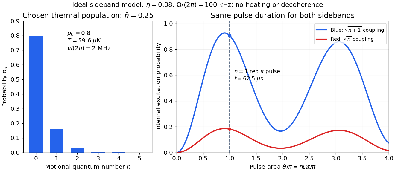
The chosen pulse gives $P_r\simeq 0.181393$ and $P_b\simeq 0.906967$. These are internal excitation probabilities, not quantum gate fidelities or cooling-cycle efficiencies. An independent matrix exponentiation of each two-state block agrees with the sine formula and preserves normalization. Summing $n=0,\dots ,79$ omits probability $r^{80}<1.21\times 10^{-56}$; because every sine squared lies between zero and one, this also bounds each omitted response. The thermal relation supplies a separate dimensional check:Here $k_B$ is the Boltzmann constant. Substitution recovers $\bar{n}=0.25$; the thermal root-mean-square expansion parameter is $\eta \sqrt{2\bar{n}+1}\simeq 0.098$. This checks the populated part of the Lamb-Dicke regime, while exponentially rare large $n$ still exceed any fixed small-parameter criterion. The pulse is a leading-order model; it does not bound corrections from the full coupling or experimental noise.

A contact potential difference is an electrostatic electric potential difference associated with different conducting surfaces brought into electrical equilibrium. Surface condition and different work functions can create a vacuum gap field even when an external voltmeter reads zero. Connecting the metals establishes equilibrium of their electronic chemical potentials including electrostatic energy; it need not equalize the electrostatic electric potential in the gap.

The characteristic ordinary differential equations $\dot{x}=y$, $\dot{y}=x$ preserve $u=x^2-y^2$. Away from the origin, $u=x^2-y^2$, $v=2xy$ have nonzero Jacobian determinant $4(x^2+y^2)$, and the chain rule reduces the displayed equation to $2(x^2+y^2)f_v=0$. Hence locally $f=F(u)$.

Globally, a level set of $u$ can have disconnected characteristic components, permitting different profiles on its different branches. A smooth counterexample on the whole plane is $f=\exp [-1/(x^2-y^2{)}^2]$ where $x>0$ and $x^2>y^2$, and $f=0$ elsewhere. The exponential is flat on the wedge boundary, so this extension is smooth and satisfies the equation. Nevertheless the points $(1,0)$ and $(-1,0)$ have equal $u$ and different function values. One global profile $F(u)$ therefore needs an additional branch-identification condition, rather than following from the local change of variables alone.

For the linear partial differential equation $2y{u}_x-x{u}_y=0$, the method of characteristics gives $\dot{x}=2y$, $\dot{y}=-x$, $\dot{u}=0$. Thus $\varphi =x^2+2y^2$ is constant on each characteristic curve, whose nonzero level sets are ellipses. On a domain containing entire such ellipses, the solutions have the form $u=F(\varphi )$, subject to the desired regularity at the origin.

For the inhomogeneous equation $2y{u}_x-x{u}_y=xy(2y^2-x^2)$, a particular solution is $u_p=x^2{y}^2/2$, so the general solution is $u=x^2{y}^2/2+F(x^2+2y^2)$. Prescribing $u(x,1)=x^2$ fixes $F(s)=(s-2)/2$ only for $s\ge 2$. The inner ellipses $s<2$ never intersect that data line, so the boundary values leave their solution values undetermined. Smooth extensions must match the prescribed $F$ at $s=2$; choosing the same linear formula everywhere gives one polynomial extension.

A vapor whose partial pressure exceeds its vapor pressure at the local temperature; nucleation can permit condensation.

Two fluids at a stationary, freely movable interface require equal pressures when surface tension and other normal stresses are negligible. This local pressure equilibrium does not require equal temperatures or mass densities. Curvature with nonzero surface tension or an applied load changes the normal-stress balance. Comparing points at different heights also requires the hydrostatic equilibrium condition.

For $F=F_0+b(T-T_c)M^2+d^{\prime }{M}^6$ with $b,d^{\prime }>0$, the ordered minimum has $M^4=b(T_c-T)/(3d^{\prime })$. Its singular free energy is $-2b^{3/2}(T_c-T{)}^{3/2}/\sqrt{27d^{\prime }}$. Twice differentiating in temperature gives the displayed ordered-side heat capacity singularity, with mean-field critical exponent $\alpha =1/2$. This path keeps the quartic coefficient tuned to zero; a generic path with a positive quartic term instead crosses over to the ordinary quartic result.

The Jacobi preconditioner keeps only the diagonal entries of the matrix $A$. For a symmetric positive-definite matrix, these entries are positive, so its auxiliary solve is $z_i=r_i/a_{ii}$. It rescales coordinates with very different diagonal sizes, but cannot remove arbitrary off-diagonal coupling.^[ref]

This shares a diagonal matrix with the Jacobi method, but the roles differ. The Jacobi method specifies a whole stationary iterative method for a linear system; a Jacobi preconditioner supplies an auxiliary solve to another iterative method, including the Preconditioned conjugate gradient method.

A matrix all of whose entries are zero. It is the additive identity among matrices of the same dimensions and represents the zero linear map in any choice of bases.

The matrix dimensions $r\times c$ specify the number of rows and columns of a matrix. For matrix multiplication, an $r\times s$ matrix can multiply an $s\times t$ matrix, yielding an $r\times t$ matrix product.

The matrix entry $a_{ij}$ is the value in row $i$ and column $j$ of a matrix $A$.

Multiplying the upper-level and photon equations by $h{\nu }_0$ makes the cancellation of internal transfer visible:Incoming excitation becomes unused excitation carried away, internal dissipation, useful output, or a change in stored energy. Translational kinetic energy, the source's other internal states and preparation losses lie outside this two-level budget. The output cannot exceed the incoming excitation power $h{\nu }_{0}F$.

Choose $G=10^{-4}{\mathrm{s}}^{-1}$ per unit inversion, $\gamma =10^4{\mathrm{s}}^{-1}$, ${\kappa }_{\mathrm{int}}={\kappa }_{\mathrm{out}}=10^6{\mathrm{s}}^{-1}$, and $F=4\times 10^{14}{\mathrm{s}}^{-1}$. These are stipulated teaching parameters. Then $N_0=4\times 10^{10}$, $F_{\mathrm{th}}=2\times 10^{14}{\mathrm{s}}^{-1}$, $N_{\mathrm{ss}}=2\times 10^{10}$ and $n_{\mathrm{ss}}=5\times 10^7$. Using the rounded ammonia inversion transition frequency, the loaded quality factor is approximately $7.50\times 10^4$. The incoming excitation power is $6.327\mathrm{nW}$: $4.745\mathrm{nW}$ leaves unused, $0.791\mathrm{nW}$ becomes internal dissipation and $0.791\mathrm{nW}$ is useful output, with rounding in these displayed values.

There is an instructive extraction optimum within this model. With the same $F$, $G$ and $\gamma$, put $\rho ={\kappa }_{\mathrm{out}}/{\kappa }_{\mathrm{int}}$ and $p=FG/(\gamma {\kappa }_{\mathrm{int}})=4$. For $0\le \rho <p-1$,Differentiation gives ${\rho }_{\mathrm{opt}}=\sqrt{p}-1=1$. At zero coupling no power is extracted; at $\rho =3$ the device reaches onset and the nonzero branch disappears. The optimum balances extraction against the inversion required to compensate that extraction. Equal residence rates and loss of molecular phase memory are simplifying assumptions; the calculated efficiency is not a universal bound for beam masers.

A switching-current distribution of a Josephson junction records the bias electric current at the first detected transition to a sustained nonzero electric potential difference. Interpret it using a stipulated monotone ramp $dI/dt=r>0$, a reproducible initial trapped state, and an instantaneous escape hazard function $\Gamma (I)$. Neglect retrapping and readout delay. The survival function $S$ obeys $dS/dt=-\Gamma S$, so changing variable from time to electric current givesHere $p$ is a probability density function per unit electric current, not a rate per unit time. Division by the surviving population is essential: only trials still trapped can escape. A typical switching current is consequently not identical to the noiseless superconducting critical current.

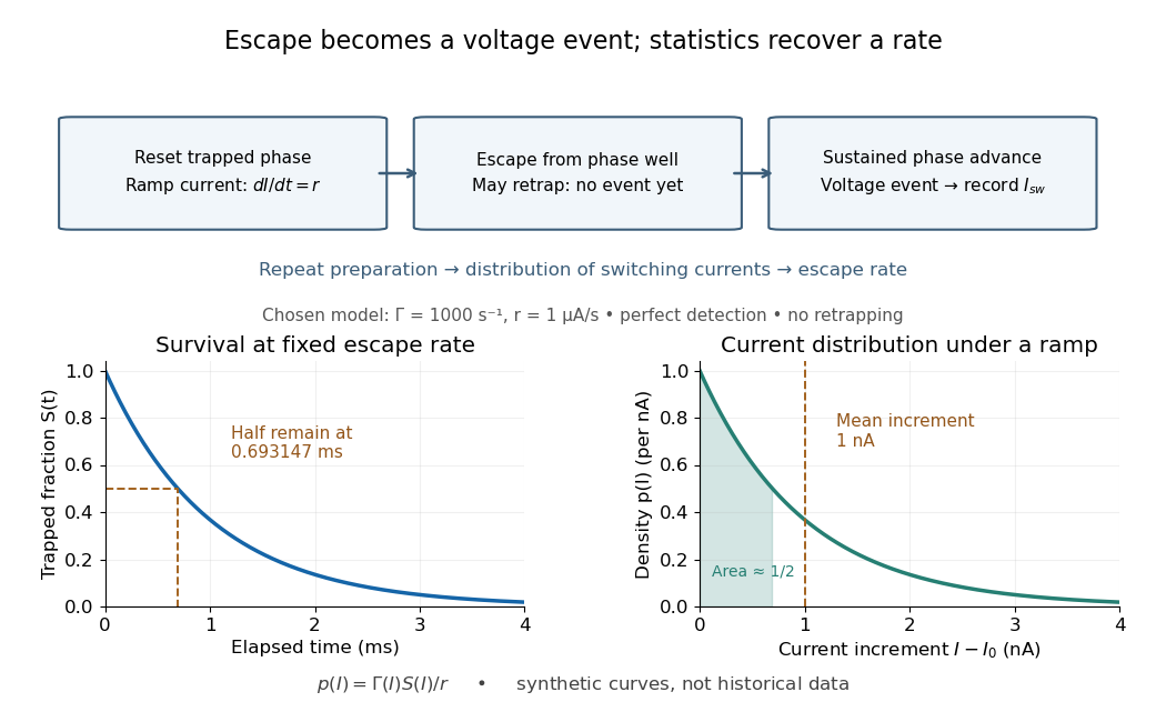
For an independent illustrative check, choose constant ${\Gamma }_0=1000{\mathrm{s}}^{-1}$ and $r=1\mu \mathrm{A}{\mathrm{s}}^{-1}$. ThenHalf the trials have switched after $\ln 2/{\Gamma }_0=0.693147\mathrm{ms}$, corresponding to $0.693147\mathrm{nA}$ of ramp. Doubling $r$ doubles the mean increment without changing the underlying escape rate. Real junction rates vary sharply with bias; this example isolates the statistical conversion.

Repeating the preparation, measuring the ramp, resolving the voltage onset, and allowing cooling after each dissipative event are prerequisites for this interpretation. Missed events, finite detection delay, changing temperature and retrapping alter the measured distribution. Even a correctly reconstructed rate needs the independent thermal and spectral checks before identifying its escape mechanism.

Two distinct Majorana fermion operators with $\{{\gamma }_i,{\gamma }_j\}=2{\delta }_{ij}$ define the displayed fermionic annihilation operator. Direct multiplication gives $f^2=0$ and $\{f,f^{†}\}=1$. Its number operator is a projection operator with eigenvalues zero and one. An individual Hermitian Majorana operator has ${\gamma }_i^{†}{\gamma }_i={\gamma }_i^2=1$, so that expression is not a nontrivial occupation observable. The occupation belongs to a chosen pair. A quadratic coupling $iJ{\gamma }_a{\gamma }_b=J(2f^{†}f-1)$ splits the pair's two occupations by $2|J|$.

Combine the material surface element evolution law with the product rule for $\mathbf{B}\cdot d\mathbf{S}$. The result isExpanding the curl gives the equivalent title formula. The ideal magnetohydrodynamic induction equation and Gauss's law for magnetism make the integrand zero and prove magnetic flux freezing, without requiring incompressible flow.