Topics (384k) Articles (398k) Users (410) Discussions (242) Comments (383) Files (13k) New article
For the convention used in light-emitting diode efficiency, the internally generated photon rate divided by the rate of electron and electron hole pairs reaching the emitting layer. Its denominator must be stated when comparing measurements.
The Liénard-Wiechert field is the electric field and magnetic field obtained from the retarded potentials of a moving point charge. In the nonrelativistic radiation zone, the electric radiation field is at retarded time. Its outgoing Poynting vector integrates to the Larmor formula. Coulomb and induction fields must also be retained when a near-field calculation is required.
State-counting and helicity factors in pion decay by  Codex 0 Created 2026-10-18 Updated 2026-11-05
In a box-normalized treatment of negative-pion two-body decay with a massless antineutrino, . The simple density of states is therefore proportional to . The spin-zero two-body helicity selection requires positive charged-lepton helicity, whose left-chiral weight is . Since , the energy factors cancel in the product and give the standard relative rate proportional to . A Lorentz-invariant phase-space measure distributes normalization factors differently but gives the same observable ratio when the amplitude is normalized consistently.
Sharp bounds from binary conditional probabilities by Codex 0 Created 2026-10-18 Updated 2026-10-25
Codex 0 Created 2026-10-18 Updated 2026-10-25Write , and . The law of total probability gives the displayed convex combination. With fixed and free in ,With fixed and free in ,The joint cell masses are nonnegative and sum to one, proving sharpness in the joint-model interpretation. For ordinary conditional probabilities, a conditioning event must have positive mass. If both and are specified by ratios, then : for the last bounds are strict and their endpoints are the infimum and supremum. If , the marginal equals that common value for every . Endpoint mixtures remain meaningful if the unused zero-mass conditional is treated as a prescribed conditional model rather than a defined ratio.
For and , a bounded harmonic function that vanishes on the straight edges and has outer boundary data has coefficientsThis follows by separation of variables and Fourier orthogonality. Negative radial powers are excluded by boundedness at the vertex. Reflection-symmetric data have only odd Fourier modes. Knowing the resulting solution on the bisector determines all these odd coefficients by its radial power series. Without reflection symmetry, the even angular modes vanish on the bisector and cannot be recovered from that restriction alone.
Suppose , , are independent and identically distributed with Laplace distribution , where . For realized values , the likelihood function and log-likelihood function areFor fixed , maximum likelihood estimation of the location therefore minimizes the sum of absolute losses. This connects the Laplace distribution to robust statistics: each observation contributes a cost growing linearly with its distance, whereas squared-error loss grows quadratically.
Why does a sample median minimize ? Between successive order statistics, moving a little to the right increases each distance to a value on the left and decreases each distance to a value on the right. Hence the slope is the number on the left minus the number on the right. It changes from negative to positive at the middle. More precisely, if , all minimizing locations areFor an even sample size, the objective is flat throughout the interval between the two central order statistics. The midpoint convention for the sample median selects one solution; it does not prove uniqueness. [ref]
Laplace (Double Exponential, Bilateral Exponential) Distribution. SciPy 1.18.0 documentation; SciPy reference guide, Laplace distribution, ML location estimator and the even-N interval between the two central order statistics
This is the finite-sample counterpart of median minimizes expected absolute loss.If , maximizing over givesThe derivative is positive below this value and negative above it. Moreover the maximized likelihood function is proportional to wherever , so the same minimizing locations give the joint maximum-likelihood estimates. [ref]
1.3.6.6.12. Double Exponential Distribution. NIST and SEMATECH e-Handbook of Statistical Methods; NIST/SEMATECH e-Handbook, Section 1.3.6.6.12, Parameter Estimation; median and average absolute deviation formulas
The scale estimate divides by ; this formula is not an assertion that it is an unbiased estimator.The boundary case matters: if all observations equal , choose . Then and as . There is no finite joint maximum-likelihood estimate in the parameter space . In particular, this always occurs for . Writing does not produce an admissible Laplace distribution.
At eigenvalue zero the Laguerre differential operator on polynomials gives , equivalently . Thus and the displayed solutions follow from the exponential integral. For any , all solutions with can be written . The choices and are linearly independent despite sharing that one prescribed value.
The second branch grows as at infinity and has a logarithmic singularity at zero. It is consequently excluded from the regular weighted square-integrable eigenproblem with weight . Only the constant zero mode remains in that self-adjoint realization. A normalization at one interior point alone is not enough to select a unique second-order solution.
A disjoint-set data structure stores the current partition of a set of vertices into connected components of a graph. The operation returns a representative of the block containing . Two vertices are in the same block exactly when their representatives agree. For each candidate edge , compare and . Equal representatives mean reject; different representatives mean accept and perform , merging the two blocks. The representatives are bookkeeping choices, not preferred vertices of the minimum spanning tree.
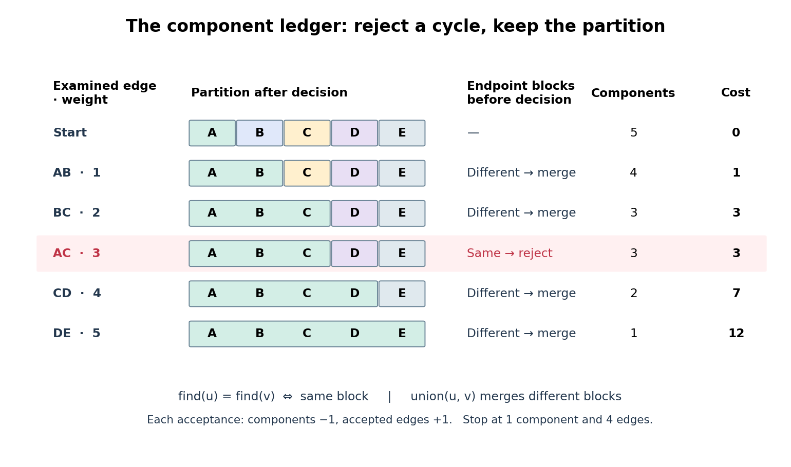
Connected components of a graph merge only when an edge is accepted
. The same example as a disjoint-set data structure ledger. Each coloured band is one block of the current partition of a set. The rejection of leaves both the partition of a set and the running cost unchanged. Bands show membership, not internal representative pointers. Details.Every acceptance reduces the connected component of a graph count by one and increases the accepted edge count by one, preserving . Thus the ledger reaches exactly when . Only ten representative queries and four merges are needed for the five examined edges, counting two queries per examination and using the already found representatives for each merge. Neither breadth-first search nor reconstruction of a graph path is needed for these connectivity queries.
For and , comparison sorting algorithm takes time for , using Big O notation. One simple disjoint-set data structure implementation stores each block as a rooted tree and attaches the smaller block's root below the larger block's root. Whenever a vertex's depth increases, its block size at least doubles, so its depth is at most . Consequently each representative query or merge takes time. Initialization plus the scan costs ; including sorting algorithm gives , hence for a connected input with . These are operation bounds, not measured timings.[ref]
WeightedQuickUnionUF.java. Robert Sedgewick and Kevin Wayne, Algorithms, 4th edition, companion WeightedQuickUnionUF.java: class documentation and union method; union by size without path compression, linear initialization and logarithmic operations
An edge is safe for the current accepted forest if some minimum spanning tree contains both and that edge. The loop invariant is that some minimum spanning tree contains every accepted edge. It holds initially for the empty edge set. Suppose the next accepted edge joins a current connected component of a graph to its complement. No earlier rejected edge crosses this cut of a graph: once its endpoints are in one connected component of a graph, subsequent merges never separate them. Thus is a lightest edge across that cut of a graph.
For the short exchange argument, take a minimum spanning tree containing . If is absent, adding it creates a fundamental cycle. This graph cycle contains another edge crossing the same cut of a graph. No edge of crosses the cut of a graph, so is not in . Replace by : the result is a spanning tree containing and , with no greater total weight because . It is therefore also a minimum spanning tree. This is the minimum spanning tree cut property in the form needed for tied weights.
In the example, is safe after rejecting : the current connected component of a graph has crossing edges of weights . Its cheapest connection is . The rejected is also the unique heaviest edge of the graph cycle , so the minimum spanning tree cycle property excludes it from every optimum.
Negative and zero edge weights are allowed: the comparisons and exchange argument still apply. Ties can give several minimum spanning trees, though they need not; any order among equal-weight edges remains valid. Distinct edge weights guarantee a unique minimum spanning tree. To see why, take the lightest edge belonging to exactly one of two proposed optima, say . Deleting from gives a cut of a graph; the other optimum has a graph path across it, containing an edge absent from . Hence , and replacing by improves that other optimum, a contradiction. For disconnected input, process all edges to obtain a minimum spanning forest, one minimum spanning tree per original connected component of a graph; no spanning tree of the whole graph exists.[ref]
KruskalMST.java. Robert Sedgewick and Kevin Wayne, Algorithms, 4th edition, companion KruskalMST.java, class documentation and constructor: arbitrary signed weights, ties, disconnected input and sorted processing
Consider this original connected graph on vertices . Its undirected edges, already in increasing weight order, areHere means the unordered pair ; the weights are dimensionless costs. Accept and , with total . Reject : its endpoints already have the graph path , so it would close the graph cycle . Accept and , reaching all five vertices with four edges. The resulting minimum spanning tree isStop here: and need not be examined. If processing continued, both would be rejected because their endpoints are already in the same connected component of a graph.
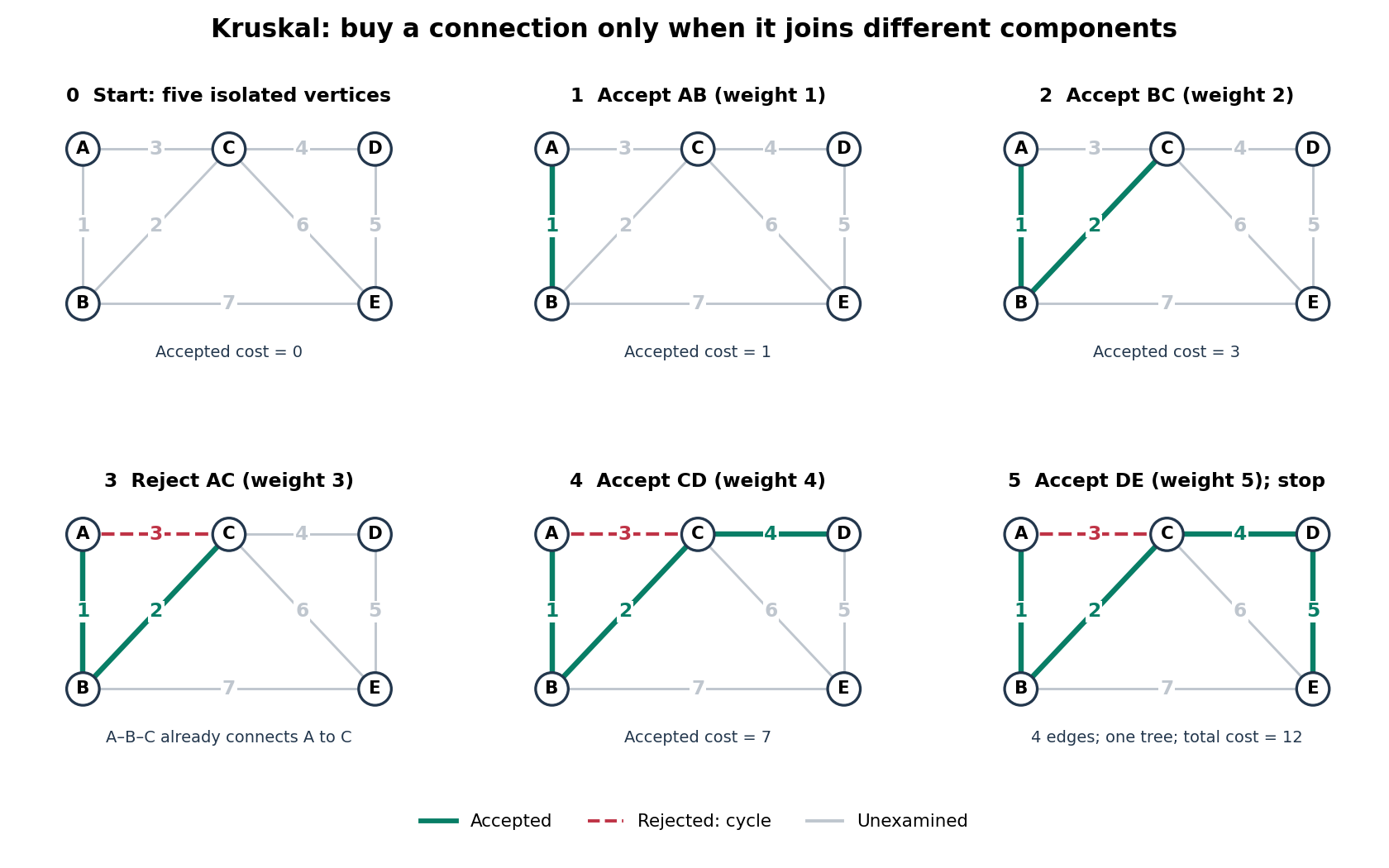
Taking the three cheapest edges instead gives a graph cycle on , leaving isolated: it is neither a forest nor a spanning tree. Even taking the four cheapest edges adds only and leaves isolated. A cheap infeasible selection cannot compete with a minimum spanning tree. For this small graph, checking all four-edge subsets gives a direct certificate: among those that are spanning trees, exactly one has minimum cost , namely . The general algorithm avoids this exhaustive search.
For a rod with unit mass density and elastic modulus, the Kelvin-Voigt model gives , . For the operator with the opposite overall sign, , the inverse under the Fourier transform convention is the displayed expression. Its poles are . With real, the retarded fundamental solution in spatial Fourier variables is . Its initial derivative is , fixed by the leading coefficient . At a repeated root take the continuous limit; for imaginary the sine becomes a hyperbolic sine.
The physical Jeans length is . A pressureless uniform sphere of initial density has free-fall time of a uniform sphere , giving the title relation. Thus a full-wavelength sound-crossing time and this exact free-fall convention agree in scaling, not numerical value. Using the scale instead gives , the inverse long-wave static Jeans growth-rate spectrum limit. At the threshold itself pressure balances gravity and the net growth rate vanishes; the pressureless free-fall time must not be confused with that marginal mode's infinite growth time.
A strictly diagonally dominant matrix guarantees convergence of the Jacobi method for every initial vector.[ref]
Notes for Ma221 Lecture 21, Nov 10 2009. Math 221, Matrix Computations, Fall 2009; Theorem 1 on strict row diagonal dominance and its proof beginning “Split A = D − (D − A)”
Indeed, using the maximum norm , the induced operator norm is the largest absolute row sum. The Jacobi method has and for , soThis gives a cheap sufficient check without computing any eigenvalues. For the Jacobi iteration for a three-variable tridiagonal system, the absolute row sums of are , giving . The true spectral radius gives a sharper eventual rate.
Strict diagonal dominance is sufficient, not necessary: violates it in the first row, but its Jacobi method has eigenvalues and converges. Conversely, being a positive-definite matrix alone is insufficient: the Jacobi convergence for a three-by-three equicorrelation matrix with has positive eigenvalues for , but spectral radius for its iteration matrix. The extra tridiagonal matrix structure in Jacobi convergence for a symmetric positive-definite tridiagonal matrix is therefore substantive.
Consider the original linear system with a symmetric matrix that is also a tridiagonal matrix:Here and the Jacobi method readsStarting from , the first three vectors areEvery right-hand side uses superscript , including the middle row, even when a new first coordinate has already been computed.
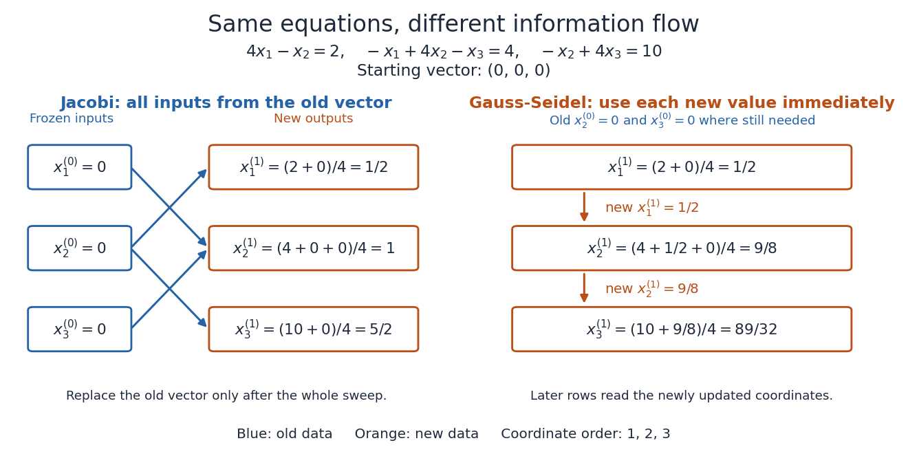
Simultaneous old-to-new component updates in the Jacobi method, compared with immediate reuse in the Gauss-Seidel method
. Details. For comparison, a first Gauss-Seidel method sweep in coordinate order givesThe new first coordinate enters the middle update, and the new second coordinate enters the final update. Accidentally overwriting old coordinates during a Jacobi method sweep therefore changes the mathematical method.
The linear-system residual is computable without knowing . The forward error is the actual difference from the desired solution. For an invertible matrix,Keeping fixed, the approximate vector exactly solves with . Thus, for , is the relative backward error when only the right-hand side may change. For a vector norm and its induced operator norm,A small relative linear-system residual ensures a small relative forward error when the condition number is moderate; an ill-conditioned matrix can amplify it. The bound follows directly from and .[ref]
2.8 Conditioning of linear systems. Fundamentals of Numerical Computation by Tobin A. Driscoll and others; §2.8.1, Theorem 2.8.1, equation (2.8.6), right-hand-side perturbation bound applied with Δb = −r
For the Jacobi iteration for a three-variable tridiagonal system, the first linear-system residual is , while the first forward error is . In the Euclidean norm, the relative forward error is and the relative linear-system residual is . Its spectral condition number of a positive-definite matrix is , so the bound is about . The bound is a guarantee, not an equality. In floating-point arithmetic, recompute the linear-system residual from the current vector when checking termination; a small update alone need not certify a small forward error.
A stationary iterative method for a linear system converges to its specified fixed point for every initial vector if and only if its iteration matrix satisfies , where the spectral radius is the largest modulus of an eigenvalue.[ref]
Notes for Ma221 Lecture 21, Nov 10 2009. Math 221, Matrix Computations, Fall 2009; Basic iterative methods: theorem following the spectral-radius lemmas, before the Jacobi update
For a diagonalizable matrix, write . Then , so each eigenvector coefficient tends to zero exactly when its eigenvalue has modulus less than one. For a general matrix, the Jordan normal form gives the same result: a Jordan block with a nilpotent matrix of size satisfiesIf , every coefficient tends to zero because exponential decay beats any fixed polynomial in ; if , the block vanishes once . Conversely, an eigenvector with provides an initial error that cannot tend to zero. For a real matrix with complex eigenvalues, the same obstruction appears in the real invariant subspace spanned by the real and imaginary parts of an eigenvector.
The words "every initial vector" matter. For example, fails the criterion, but still tends to zero. Here a generic initial error has a nonzero first coordinate and diverges; the exceptional errors lie on the second coordinate axis. With , generic errors oscillate rather than diverge in norm, while the same exceptional axis still converges. Both are valid matrix splittings with and . In general the convergent errors form the direct sum of the generalized eigenspaces for ; if , this is a proper linear subspace.
A small spectral radius describes eventual convergence, but does not imply that the Euclidean norm of the error decreases on every step for a non-normal matrix. An operator norm bound does give the stepwise estimate . For a real symmetric matrix, the matrix 2-norm equals its spectral radius, making this particularly direct.
Here is the volume of the unit ball in -dimensional Euclidean space. Rotational invariance makes the integral an isotropic tensor, while complete symmetry in its four indices equates the three coefficients. Contracting and gives times their common value. The same contraction of the integral is , proving the formula. For the coefficient is . This is the fourth-order counterpart of the isotropic second moment of a ball.
In three-dimensional Euclidean space, a rank-three tensor invariant under every proper rotation is a scalar multiple of the Levi-Civita symbol. The distinction between proper rotations and all orthogonal transformations matters: . A polar tensor of odd rank invariant under every orthogonal transformation must vanish, since the transformation changes its sign. A nonzero invariant rank-three object under reflections is instead a pseudotensor, whose transformation law includes the extra determinant factor.
For steady Isothermal Bondi accretion from gas at rest at infinity, define , and , where . The Bernoulli function and mass conservation give . The left side has minimum at , and the radius-dependent part on the right has minimum two at . Existence over all positive radii therefore requires the displayed bound. Equality permits the smooth accelerating-inward transonic branch and gives the usual isothermal Bondi accretion rate. Smaller positive rates have an everywhere-subsonic reservoir-connected branch, and zero rate gives a hydrostatic atmosphere. An absorbing inner boundary inside the sonic radius selects the critical inflow; steady isothermal equations and the outer density alone do not specify that inner condition.
Pinned article: Introduction to the OurBigBook Project
Welcome to the OurBigBook Project! Our goal is to create the perfect publishing platform for STEM subjects, and get university-level students to write the best free STEM tutorials ever.
Everyone is welcome to create an account and play with the site: ourbigbook.com/go/register. We belive that students themselves can write amazing tutorials, but teachers are welcome too. You can write about anything you want, it doesn't have to be STEM or even educational. Silly test content is very welcome and you won't be penalized in any way. Just keep it legal!
Intro to OurBigBook
. Source. We have two killer features:
- topics: topics group articles by different users with the same title, e.g. here is the topic for the "Fundamental Theorem of Calculus" ourbigbook.com/go/topic/fundamental-theorem-of-calculusArticles of different users are sorted by upvote within each article page. This feature is a bit like:
- a Wikipedia where each user can have their own version of each article
- a Q&A website like Stack Overflow, where multiple people can give their views on a given topic, and the best ones are sorted by upvote. Except you don't need to wait for someone to ask first, and any topic goes, no matter how narrow or broad
This feature makes it possible for readers to find better explanations of any topic created by other writers. And it allows writers to create an explanation in a place that readers might actually find it.
Figure 1. Screenshot of the "Derivative" topic page. View it live at: ourbigbook.com/go/topic/derivativeVideo 2. OurBigBook Web topics demo. Source. - local editing: you can store all your personal knowledge base content locally in a plaintext markup format that can be edited locally and published either:This way you can be sure that even if OurBigBook.com were to go down one day (which we have no plans to do as it is quite cheap to host!), your content will still be perfectly readable as a static site.
- to OurBigBook.com to get awesome multi-user features like topics and likes
- as HTML files to a static website, which you can host yourself for free on many external providers like GitHub Pages, and remain in full control

Figure 2. You can publish local OurBigBook lightweight markup files to either OurBigBook.com or as a static website.
Figure 3. Visual Studio Code extension installation.
Figure 5. . You can also edit articles on the Web editor without installing anything locally. Video 3. Edit locally and publish demo. Source. This shows editing OurBigBook Markup and publishing it using the Visual Studio Code extension. 
- Infinitely deep tables of contents:




All our software is open source and hosted at: github.com/ourbigbook/ourbigbook
Further documentation can be found at: docs.ourbigbook.com
Feel free to reach our to us for any help or suggestions: docs.ourbigbook.com/#contact