Topics (384k) Articles (398k) Users (410) Discussions (242) Comments (383) Files (13k) New article
Take a proper rotation matrix with real number entries. Then hasThis odd linear orbital model has an isotropic gap magnitude. Isotropic gap magnitude does not require s-wave pairing: the spin components can rotate together with the orbital direction. Nor does the magnitude fix the relative spin-orbit orientation represented by .
For both displayed models, . The triplet gap matrix , written with Pauli matrices, satisfiesThus these models give the same gap magnitude for the two spin branches. That last simplification would fail for a general complex triplet vector with a nonzero cross product. The displayed angular curves illustrate these specified matrices; they are not a microscopic derivation of the phase diagram.
Take a real unit vector in spin space and choose orthogonal orbital axes. The model hasIt vanishes at the two polar directions and is largest at the equator. The orbital factor changes sign when is reversed, as required for the odd orbital part of spin-triplet p-wave pairing. Calling the phase A does not mean its order parameter is one real number.
A spin-zero parent at rest decaying to two particles requires their helicities to be equal. Choosing particle 1 along and particle 2 along gives total projection . In negative-pion decay, the massless antineutrino has positive helicity, so the negative charged lepton must also have positive helicity. This is the suppressed component for a left-chiral weak charged current.
A counterflow heat exchanger sends two streams in opposite directions along a common exchange region. The separating wall transmits heat while the streams remain physically distinct. This arrangement lets the hot inlet interact with the already warmed cold outlet, and the hot outlet interact with the cold inlet, maintaining a driving temperature difference over the length.
For steady operation with negligible losses and no external work, the hot stream's lost enthalpy equals the cold stream's gained enthalpy. With constant heat-capacity rates, . The cold outlet can exceed the hot outlet temperature because those outlets are at opposite ends; local passive transfer still proceeds from hotter to colder. In helium liquefaction and a dilution refrigerator, returning cold fluid precools the incoming stream, reducing the load on the final cooling stage.
A heat-current relaxation time measures the decay of a departure from equilibrium carrying heat. It need not equal the momentum relaxation time or the time between arbitrary scattering events. In an isotropic degenerate-electron estimate, . Small-angle inelastic electron-phonon scattering can remove an excitation energy of order while barely changing the electron's velocity direction, thus relaxing heat more efficiently than charge flow.
For a rapidly spinning gyrocompass with axle constrained horizontally, take azimuth positive from north towards west and positive spin angular momentum . In the terrestrial rotating reference frame, the vertical component of the torque equation, with zero external vertical torque, is . Here is the vertical moment of inertia and terms of order have been neglected. The small-angle approximation about gives simple harmonic motion with the displayed squared angular frequency. Linearizing about reverses its sign and gives an unstable equilibrium. At the poles this restoring effect vanishes. For a thin rotationally symmetric flywheel, the perpendicular axis theorem gives .
For vacuum incidence at fixed angle into a transparent isotropic medium, Snell's law gives . Thus , andAngles must be differentiated in radians. This determines the local group velocity from a first derivative of measured refraction angles; pulse broadening needs further information about group velocity dispersion and absorption.
Gibbs free-energy change for a pressure-linear gas correction by  Codex 0 Created 2026-10-18 Updated 2026-11-05
For the equation of state , integrate along an isotherm. This gives the displayed Gibbs free energy difference. Its negative temperature derivative at fixed endpoint pressures gives . The physically admissible branch must retain positive volume.
How many attempts give at least a chosen success probability ? For a positive-integer geometric distribution with , completion by attempt means , soThe logarithm is negative, which reverses the inequality when dividing. The least integer meeting the target is therefore obtained with the ceiling function:For our constructed independent retry mechanism with and ,To verify minimality directly, eight attempts give , whereas nine give . Under the zero-based convention, the same completion event is , with failure to complete given by ; saying would allow ten attempts. A 95% deadline controls a tail probability, while the expected value describes an average.
At success occurs on the first attempt, so ; the logarithm formula is inapplicable. At no finite deadline achieves a positive target. For , no finite deadline guarantees success with probability one because . A retry cap at produces the capped geometric waiting time as the number of attempts actually spent; reaching the cap can mean either success on the last allowed attempt or failure of all attempts.
Write a generalized circle equation as , where are real. Under the reciprocal Möbius transformation , with , multiply by to obtainThus the coefficient triple transforms as . A nondegenerate circle through zero has and becomes a straight line; a straight line missing zero becomes a circle through zero on the Riemann sphere. When working only with finite nonzero coordinates, retain the excluded point even if it satisfies the multiplied equation.
This reciprocal transformation is different from inversion in a circle, whose unit-circle formula is . The latter reverses orientation; the reciprocal transformation is holomorphic away from its pole.
For integers , integration by parts givesThe boundary term vanishes because at zero and Gaussian decay dominates every power at infinity. The initial values are , the half-line Gaussian integral, and by the substitution rule . More generally, for real , that substitution gives , linking the recurrence to the Gamma function.
A strictly diagonally dominant matrix or a real symmetric positive-definite matrix guarantees convergence of the Gauss-Seidel method from every initial vector. These are sufficient conditions.[ref]
Notes for Ma221 Lecture 21, Nov 10 2009. Math 221, Matrix Computations, Fall 2009; Theorem 1, strict row diagonal dominance, web lines 462–465; Theorem 3, positive-definite SOR and its ω = 1 specialization, web lines 490–493
For strict diagonal dominance, putInduct through a sweep. Old coordinates have absolute error at most ; previously updated coordinates have absolute error at most . The component update and the triangle inequality therefore bound the new error by . This proves , a maximum norm contraction.
For a symmetric positive-definite matrix, write . The Householder-John theorem applies to and , because is a positive-definite matrix. Hence the iteration matrix has spectral radius less than one, which gives the convergence criterion for a stationary iteration.
There is also a geometric reason fresh updates help: the Gauss-Seidel method is exact coordinate descent on the convex quadratic functionHolding the other coordinates fixed, minimizing in coordinate gives the corresponding row update. A change lowers by exactly . Each fresh coordinate is therefore the minimizer for the current vector, and a complete sweep lowers the quadratic form error unless every coordinate already solves its row. This explains the method's beauty without implying monotone decrease in every vector norm.
Gauss-Seidel iteration for a two-variable positive-definite system by Codex 0 Created 2026-10-18 Updated 2026-10-31
Codex 0 Created 2026-10-18 Updated 2026-10-31Consider the original linear systemDirect substitution verifies the solution. The matrix is a symmetric positive-definite matrix: completing the square in its quadratic form gives for every nonzero vector. It is also a strictly diagonally dominant matrix.
Starting from , update the first row and then the second:The first sweep gives and . The next gives and . The second row uses during the first sweep, even though the initial first coordinate was zero.
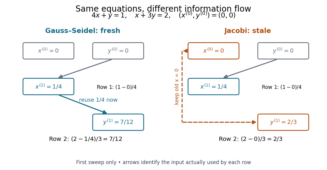
Fresh and stale inputs in the first sweep of the original two-variable linear system
. Details. With a stale first coordinate, the Jacobi method would instead give after the first sweep. Both methods have the same fixed point, but changing when coordinates become available changes the entire sequence of vectors.
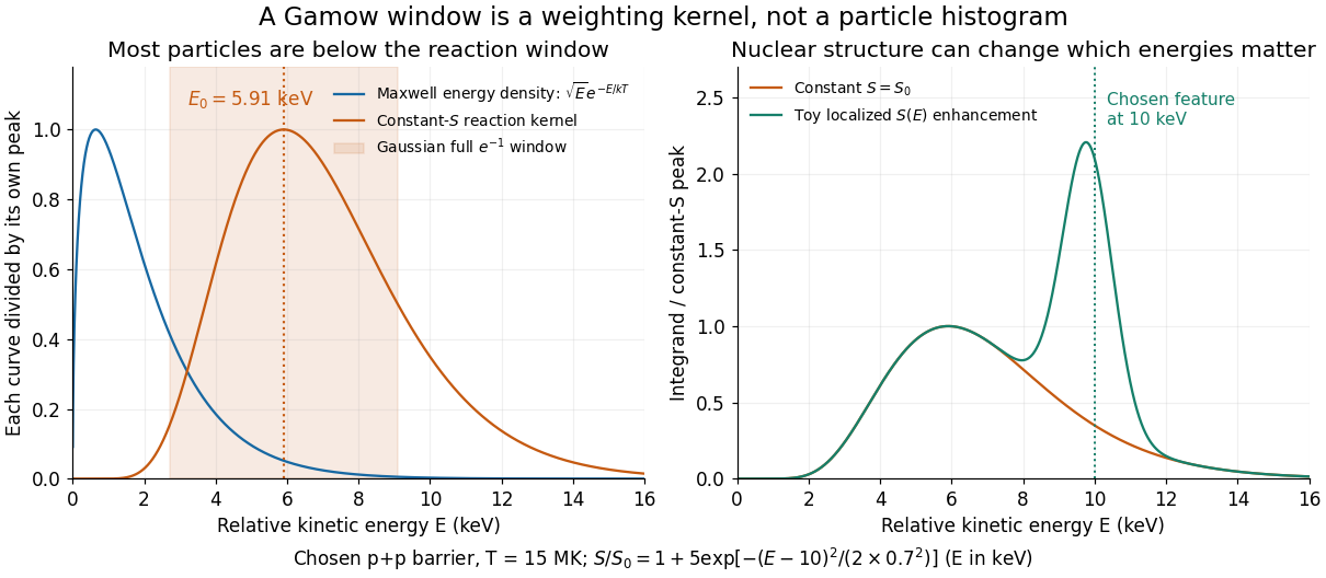
The Gaussian approximation to a nonresonant thermonuclear rate already gives the saddle and curvature. In its notation , so the same result readsThe full width joins the two points at of the peak of the approximating Gaussian function; it is neither its standard deviation nor its full width at half maximum . These are local Gaussian approximation widths, not exact equal-height endpoints of the asymmetric kernel.
Why keep the astrophysical S factor inside the integral? If is positive and smooth, stationarity of gives a leading peak displacement . The slow-variation test is therefore , together with small curvature corrections. More generally any energy-dependent prefactor shifts the saddle; a temperature-dependent prefactor also changes the local temperature exponent of a thermonuclear reaction. A sharp nuclear feature can invalidate this expansion altogether.
Choose and for an illustrative proton pair. Then , and . The relative Maxwell-Boltzmann velocity distribution has energy-density maximum , far below the reaction kernel's maximum. Now choose the deliberately artificial enhancementNumerical integration raises the rate by about at the same temperature, even though the enhancement is away from . This is a sensitivity experiment, not a claimed proton–proton nuclear level or a physical nuclear line-shape model. It illustrates why extrapolating without checking nearby structure can fail.
For fixed strict preferences, a proposer-optimal stable matching gives each proposer its best partner obtainable in any stable matching, with unmatched ranked last. The Gale-Shapley algorithm achieves all these individual optima simultaneously. In the worked example, gives partners ranked , respectively; the alternative gives them ranks .
Suppose a first rejection of a pair belonging to some stable matching occurs when rejects for . Every partner prefers to has already rejected it, so none can be its partner in . If , then prefers to , while prefers to : a blocking pair in stable matching, a contradiction. Hence no rejected pair is stable, and each proposer receives its best stable partner. Under strict preferences this also makes the outcome independent of proposal order.
Fit the positions of successive, consistently defined troughs by linear regression, . A constant intercept absorbs the contact potential difference, collection phase and initial energy effects; estimates the repeated loss expressed as a voltage. Subtracting successive positions cancels . A line fit uses every position and leaves residuals that can reveal curvature or a misidentified trough. It still assumes that the phase is constant over the fitted range and that all troughs belong to the same loss channel.
For an original numerical example, choose and synthetic positions . Their successive spacings are . The ordinary least squares formulas giveThe fitted residuals are , with zero sum and zero index-weighted sum. Their residual sum of squares is . If independent, equal-variance, zero-mean errors describe these positions, the residual variance estimate is and the slope standard error is . Thus the inferred model loss is with conditional standard error . These errors summarize only the chosen position scatter; a voltage-scale error or a drifting collection phase is not included. Adjacent spacings share a position error and are therefore correlated even when position errors are independent.
The offset has a sharper identifiability limitation. Even if a constant-phase model were exact, an initial beam kinetic energy shifts the troughs by . For the symmetric illustrative curve, . The transformation , leaves every trough position unchanged. Measuring alone therefore cannot determine the contact potential difference. Relabeling also changes by without changing . An independent offset calibration and a justified collection model are needed before turning a first trough into an excitation threshold. Varying tests this model's predicted half-voltage shift of the trough centers; it is a diagnostic prediction of this chosen curve, not a universal correction for experimental minima.
Define a signed offset so that the accelerating region adds kinetic energy . This convention concerns this gap; collector contact fields belong in the effective . An electron emitted with initial kinetic energy and undergoing identical excitation losses reaches the grid withEach loss excites a fresh chemical atom initially in its ground state. These are repeated payments of the same excitation cost. The index counts events along an electron trajectory, not the ordinal number of an atomic excited state. The outgoing energy also does not locate the last collision: after an early collision an electron can regain enough kinetic energy to cross the barrier.
At fixed , let be the normalized initial-energy probability density function within the ensemble of electrons reaching the grid, and the conditional probabilities for losses within that ensemble. Then the ideal collection law isTake and exclude paths with insufficient kinetic energy for a loss at its actual collision position. The weights contain collision positions and rates, mean free paths and angular acceptance. This equation is a bookkeeping model, not a derivation of those weights. Multiplying all incident particles by one constant transmission is an additional approximation; real transmission and can vary with .
One analytical extreme assumes , one-dimensional motion and an immediate loss whenever the kinetic energy reaches . With , and , the number of losses and remaining kinetic energy areHere is the floor function. Collection switches off for an interval of width after each reset, then recovers; the pattern repeats every . For , and , an applied gives , and rejection, whereas gives , and collection. With the dips disappear in this idealization. With no collisions, there is only a single collection onset. Both limits expose the separate roles of loss and filtering.
To draw a smooth illustrative curve, extend this periodic rule mathematically to all and convolve it with a chosen normal distribution of voltage jitter, of standard deviation :Here is the standard normal cumulative distribution function. Each summand is the smoothed indicator of the accepted interval . The result satisfies and has period . For the figure choose and plot only well beyond the startup region. This is a chosen phenomenological curve, not a Boltzmann equation transport prediction or a fit to measured electric current. Its symmetric troughs center on , rather than the reset voltages . Finite excitation rates, several loss channels, space charge, initial angular and energy spreads, and real electrode geometry can change the trough shape and phase; a single convolution does not solve these effects.
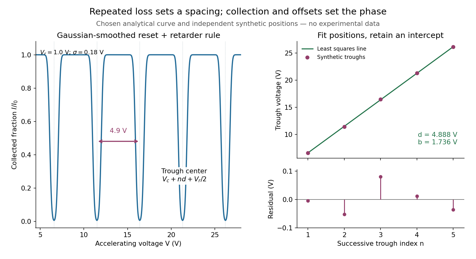
Illustrative repeated-loss collection and an independent synthetic spacing fit
. Left: the chosen Gaussian-smoothed threshold model, with , , and . Right: separately chosen synthetic trough positions, their ordinary least squares fit and residuals. The points are not extracted from the left curve or a historical trace. Source. Details.For electrons directed normally toward an ideal planar collector, a retarding electric potential difference imposes the barrier . Write its transfer as , where is the Heaviside step function and the positive elementary charge. Thus a perfectly sharp loss need not produce a sharp drop in electric current: the drop also depends on where the outgoing energy lies relative to the barrier. For an oblique incident electron at angle to the normal, the same planar model instead tests ; angular scattering can change collection even at unchanged total kinetic energy.
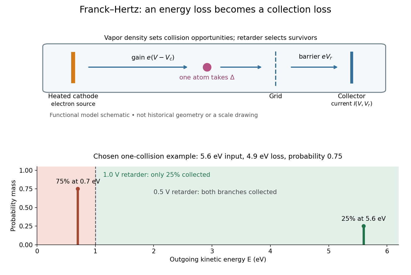
Franck-Hertz energy-loss model: separate acceleration, loss and collection
. Original functional schematic, not a scale reconstruction of a historical tube. The lower panel applies an ideal normally incident retarder to the explicitly chosen one-collision example. Equal vertical strokes mark outgoing energies; their labeled weights give probabilities. Source. Details.For example, choose a monoenergetic incoming beam with , and . After one encounter, have and have . A retarder collects only , whereas a retarder collects ; here is the incident electric current with fixed geometrical acceptance and no background. The mean outgoing kinetic energy is , independently checked by . These are chosen inputs and calculated fractions, not historical measurements.
More generally, let be the normalized outgoing probability density function at a fixed accelerating electric potential difference , for the normally incident idealization. A retarding scan givesThe second equation follows by differentiating the lower integration limit, with Dirac delta functions understood for sharp beams. It explains why an integrated collector readout can reveal an energy distribution. With angles present it probes the distribution of normal kinetic energy; finite instrumental resolution smooths it, and numerical differentiation amplifies noise. Keep the incoming beam fixed during this scan. A scan of changes itself and cannot be differentiated by the same inversion formula.
In any finite-dimensional Euclidean space, this extension is a smooth function and all its partial derivatives at the origin vanish. Away from zero, repeated differentiation gives finite sums of coordinate polynomials divided by powers of , multiplied by . Every such term is bounded in absolute value by near zero. Since Gaussian decay dominates every power, this bound tends to zero faster than any prescribed positive power of . Induction using difference quotients then proves smoothness and zero derivatives of every order at zero.
The origin is nevertheless a strict global minimum, because for . All its Taylor series coefficients vanish, so the function is not real analytic at zero. Adding a constant preserves the stationary minimum but changes the zeroth-order value. An expression written only for has no stationary point at the excluded origin until an extension is specified.
Pinned article: Introduction to the OurBigBook Project
Welcome to the OurBigBook Project! Our goal is to create the perfect publishing platform for STEM subjects, and get university-level students to write the best free STEM tutorials ever.
Everyone is welcome to create an account and play with the site: ourbigbook.com/go/register. We belive that students themselves can write amazing tutorials, but teachers are welcome too. You can write about anything you want, it doesn't have to be STEM or even educational. Silly test content is very welcome and you won't be penalized in any way. Just keep it legal!
Intro to OurBigBook
. Source. We have two killer features:
- topics: topics group articles by different users with the same title, e.g. here is the topic for the "Fundamental Theorem of Calculus" ourbigbook.com/go/topic/fundamental-theorem-of-calculusArticles of different users are sorted by upvote within each article page. This feature is a bit like:
- a Wikipedia where each user can have their own version of each article
- a Q&A website like Stack Overflow, where multiple people can give their views on a given topic, and the best ones are sorted by upvote. Except you don't need to wait for someone to ask first, and any topic goes, no matter how narrow or broad
This feature makes it possible for readers to find better explanations of any topic created by other writers. And it allows writers to create an explanation in a place that readers might actually find it.
Figure 1. Screenshot of the "Derivative" topic page. View it live at: ourbigbook.com/go/topic/derivativeVideo 2. OurBigBook Web topics demo. Source. - local editing: you can store all your personal knowledge base content locally in a plaintext markup format that can be edited locally and published either:This way you can be sure that even if OurBigBook.com were to go down one day (which we have no plans to do as it is quite cheap to host!), your content will still be perfectly readable as a static site.
- to OurBigBook.com to get awesome multi-user features like topics and likes
- as HTML files to a static website, which you can host yourself for free on many external providers like GitHub Pages, and remain in full control

Figure 2. You can publish local OurBigBook lightweight markup files to either OurBigBook.com or as a static website.
Figure 3. Visual Studio Code extension installation.
Figure 5. . You can also edit articles on the Web editor without installing anything locally. Video 3. Edit locally and publish demo. Source. This shows editing OurBigBook Markup and publishing it using the Visual Studio Code extension. 
- Infinitely deep tables of contents:




All our software is open source and hosted at: github.com/ourbigbook/ourbigbook
Further documentation can be found at: docs.ourbigbook.com
Feel free to reach our to us for any help or suggestions: docs.ourbigbook.com/#contact