Consider a uniform-density cylinder with an axisymmetric radial Fourier mode $\eta =ϵe^{ikz}$. Its displaced boundary gives a first-order surface mass density $\rho \eta$, although the interior density perturbation vanishes. The gravitational Poisson equation reduces to Laplace equation away from the interface. Regularity internally and decay externally give ${\psi }_{\mathrm{in}}=A{I}_0(kr)e^{ikz}$ and ${\psi }_{\mathrm{out}}=B{K}_0(kr)e^{ikz}$. Continuity at $R$ and the derivative jump ${\psi }_{\mathrm{out}}^{\prime }-{\psi }_{\mathrm{in}}^{\prime }=4\pi G\rho ϵe^{ikz}$, together with $I_0(\kappa )K_0^{\prime }(\kappa )-I_0^{\prime }(\kappa )K_0(\kappa )=-1/\kappa$, give the title amplitude. The prime differentiates the modified Bessel function argument. This axial mode is different from an azimuthal mode on a gravitational potential of a displaced cylindrical interface.

Inelastic neutron scattering resolves $E_i-E_f\ne 0$. Through conservation of energy, a peak at positive $\hslash \omega$ identifies an allowed excitation energy; through momentum conservation, its location in $\mathbf{Q}$ constrains the spatial variation of that excitation. A phonon is a quantum of lattice vibration; a magnon is a quantum of a spin wave. Their different couplings make energy transfer alone insufficient to identify which was created.

Bertram Neville Brockhouse's aluminium experiment rotated a large single crystal, scanning analyzer angle for neutron groups. His vanadium comparison exposed the elastic resolution. Later magnetite measurements used a magnetic field intensity test to identify magnons.^[ref]

Successive orientations sample different wave vectors; analyzer settings distinguish outgoing energies. This supplies points on a dispersion relation, rather than only an angular diffraction pattern. Finite resolution can merge neighboring excitations; background, multiple scattering and processes involving several phonons can complicate interpretation. A lattice model is a testable explanation of selected features, not a guarantee that every spectral peak has the same origin.

In neutron diffraction, coherent elastic scattering adds scattering amplitudes from regularly positioned scatterers. Since $E_f=E_i$, the neutron scattering kinematics gives $k_f=k_i=2\pi /\lambda$ andFor lattice planes of interplanar spacing $d_{\mathrm{p}}$, constructive addition requires $Q=2\pi n/d_{\mathrm{p}}$ along the plane normal. Equating these expressions proves Bragg's law:For example, stipulate $d_{\mathrm{p}}=2$ ångströms and $\lambda =2$ ångströms. The first diffraction order has $\theta =30^{\circ }$ and detector deflection $60^{\circ }$. A peak position constrains a period; its intensity also depends on the crystal basis structure factor.

Clifford Glenwood Shull describes powdered sodium chloride, a crystal monochromator, and a shielded counter recording angular counts. Inserting cadmium measured background; substantial diffuse scattering complicated peak interpretation.^[ref]

Powdering supplies many crystal orientations. Comparing the angular peaks with Bragg's law constrains crystal structure; a background estimate helps distinguish specimen peaks from unwanted counts. A two-axis diffraction instrument has no separate outgoing energy analysis, so an angular pattern alone does not separate every inelastic contribution. The richer magnetic example, including a warm/cold comparison and its limits, is the manganese monoxide neutron diffraction experiment. Its extra peaks reveal magnetic order beyond the chemical periodicity; the associated magnetic neutron diffraction model is developed there.

Treat the incident and outgoing neutrons as free nonrelativistic particles outside the specimen. Their wave vectors, de Broglie wavelengths, momenta and kinetic energies obeyHere $k_i=|{\mathbf{k}}_i|$, $k_f=|{\mathbf{k}}_f|$, $m_n$ is the neutron mass, and $\hslash =h/(2\pi )$ uses the Planck constant. Subtracting the outgoing projectile quantities from the incoming ones gives the momentum transfer and energy delivered to the specimen:Thus $\mathbf{Q}$ has units of inverse length, rather than momentum. A positive $\omega$ means the specimen gains energy; negative $\omega$ means it supplies energy to the neutron. If the angle between incident and outgoing propagation directions is $2\theta$, the law of cosines givesKnowing the detector angle alone therefore leaves $Q$ undetermined unless the outgoing energy is known or an elastic scattering assumption is justified.

For a reproducible unit conversion choose $m_n=1.67492750056\times 10^{-27}\mathrm{kg}$, $h=6.62607015\times 10^{-34}\mathrm{J}\mathrm{s}$ and $1\mathrm{eV}=1.602176634\times 10^{-19}\mathrm{J}$. The first is a recommended central value; the latter two conversions are exact.^[ref] With $1$ ångström equal to $10^{-10}\mathrm{m}$ and $1\mathrm{meV}=10^{-3}$ electronvolts, substitution into $E=h^2/(2m_n{\lambda }^2)$ givesSquare brackets here mean the numerical value in the indicated unit. For an original chosen example, ${\lambda }_i=2$ ångströms and ${\lambda }_f=2.5$ ångströms give $E_i\simeq 20.451\mathrm{meV}$, $E_f\simeq 13.089\mathrm{meV}$ and $\hslash \omega \simeq 7.362\mathrm{meV}$. At $2\theta =60^{\circ }$, $Q\simeq 2.879{\mathring{\mathrm{A}}}^{-1}$. These values stipulate an allowed projectile geometry; they do not assert that any particular specimen has an excitation there.

Neutron spectroscopy measures neutron energies or the energy changes caused by interactions with a sample. In inelastic scattering, comparing incident and outgoing energy and momentum probes excitations and motion in matter rather than only its static arrangement.

A pulsed or velocity-selected beam, a sample and detectors at known directions form a typical experiment. For a nonrelativistic outgoing neutron traveling known distance $L$ from the sample in time $t$, time of flight gives $E_f=m_n{L}^2/(2t^2)$. A known incident energy then determines the sample's energy transfer. Timing resolution, flight-path uncertainty and background limit the result. ^[ref]

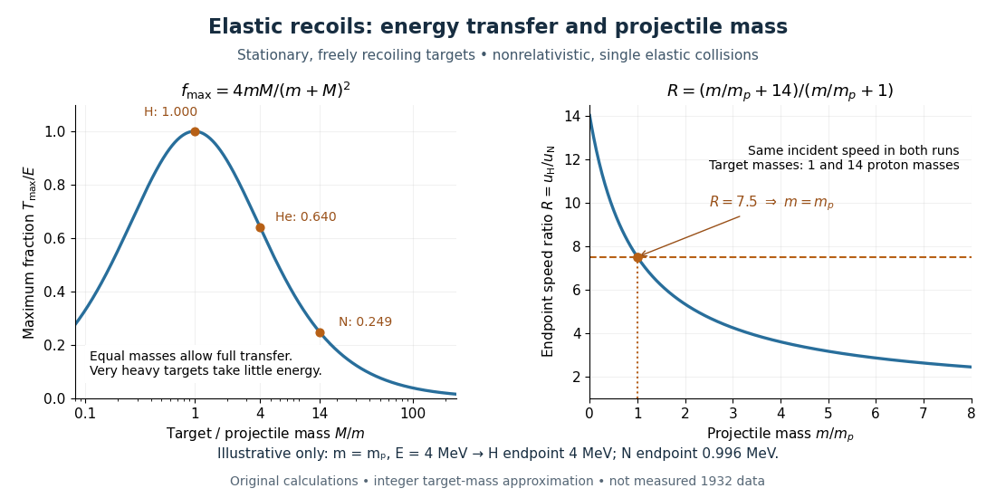
A single recoil endpoint leaves a tradeoff between incident speed and projectile mass. Two targets can remove the unknown incident speed. Assume both runs sample the same maximum projectile speed $v$ and that single elastic collisions reach the endpoint. For initially stationary target masses $M_1<M_2$, let their maximum recoil speeds be $u_1,u_2$. The maximum elastic recoil energy fraction calculation givesIf energies rather than speeds are inferred, use $R=\sqrt{T_{1,\max }{M}_2/(T_{2,\max }{M}_1)}$. The energy ratio itself is not the speed ratio.

For the stipulated $4\mathrm{MeV}$ example, hydrogen and nitrogen giveThe inferred mass then determines $v=u_1(m+M_1)/(2m)$. Changing the assumed mass to improve one recoil endpoint changes the prediction for the other: this is the constraining power of the comparison.

James Chadwick's June paper instead used approximate endpoints $u_p=3.3\times 10^{7}m/s$ and $u_N=4.7\times 10^{6}m/s$, obtaining $m/m_p\simeq 1.15$; it allowed roughly ten percent uncertainty in $u_N$. This was a rough mass comparison.^[ref]

The inverse calculation has useful built-in checks. A positive finite mass requires $1<R<M_2/M_1$. As $R$ approaches $1$, distinguishing large projectile masses becomes difficult. Differentiation givesUncertain recoil endpoints therefore produce an uncertain inferred mass; the collision model cannot turn imprecise range measurements into exact spectroscopy. If different target runs select different incident energy groups, the common-$v$ cancellation also fails.

For comparison, Compton scattering of a photon of energy $E_{\gamma }$ from a stationary free target of mass $M$ has the exact relativistic endpointThis follows by combining momentum conservation with the target's relativistic energy, maximizing transfer when the photon reverses direction. Unlike the massive-projectile calculation, this equation does not approximate the incident photon as a nonrelativistic particle.

As a separate, explicitly hypothetical test, take $m_p{c}^2=938\mathrm{MeV}$ and target rest energies $938\mathrm{MeV}$ and $14\times 938\mathrm{MeV}$. To reproduce the stipulated hydrogen recoil endpoint $T=4\mathrm{MeV}$, the photon would need $E_{\gamma }\simeq 45.36\mathrm{MeV}$. The same photon would give the heavier target at most $0.311\mathrm{MeV}$, whereas the stipulated massive projectile gave $0.996\mathrm{MeV}$. This is the structure of a two-target discrimination, not a transcription of a 1932 measurement. Actual radiation can contain more than one energy group or both photons and neutrons; a useful model must account for the observed endpoints and their origin together.

Let a projectile have mass $m$, incident speed $v$, and incident kinetic energy $E=m{v}^2/2$. The stationary target has mass $M$. In a head-on elastic collision, the signed outgoing projectile velocity $v^{\prime }$ and target velocity $u$ obey momentum conservation and conservation of energy:Factor the second equation and eliminate $Mu=m(v-v^{\prime })$. The nontrivial collision branch has $u=v+v^{\prime }$, henceThis is the maximum over scattering angles, not the energy of every recoil. To see the bound without assuming a head-on event, set the recoil momentum magnitude to $q$ and its laboratory angle to the incident direction to $\theta$. Conservation of energy with outgoing projectile momentum $\mathbf{p}-\mathbf{q}$ givesThus $T=T_{\max }{\cos }^2\theta$ for a nonzero recoil, and the endpoint occurs at $\theta =0$.

For an original numerical example, stipulate $E=4\mathrm{MeV}$ and $m=m_p$, with $m_p$ the proton mass. Approximate hydrogen, helium and nitrogen target masses by $M=m_p$, $4m_p$ and $14m_p$ respectively. Their maximum fractions and recoil energies areThese stipulated values illustrate the approximation $m_n=m_p$; they are not measurements from 1932. With $m_p{c}^2\simeq 938\mathrm{MeV}$, the incident ratio $E/(m_p{c}^2)\simeq 0.0043$ gives $v/c\simeq 0.092$, consistent with the nonrelativistic limit used here. A million electronvolts is an energy unit, whereas a mass expressed in $\mathrm{MeV}/c^2$ requires the factor $c^2$ when inserted into an energy equation.

The hydrogen endpoint permits essentially complete transfer because the projectile and target masses match. For a very heavy target, $M\gg m$, the fraction approaches $4m/M$, which is small: the target can take substantial momentum with little kinetic energy. The exact inequality follows from $(m-M{)}^2\ge 0$, which implies $(m+M{)}^2\ge 4mM$.

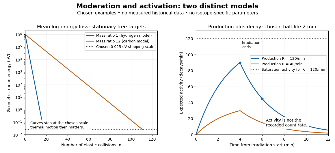
Let $\overline{N}$ be the expected value of the number of radioactive product atomic nuclei, initially zero, produced at constant rate $R$. Let their nuclear decay constant be $\lambda >0$. Assume one product species, negligible target depletion and negligible capture by the product. During irradiation, production adds $Rdt$ while radioactive decay removes $\lambda \overline{N}dt$ in expectation. Multiplying the resulting ordinary differential equation by $e^{\lambda t}$ givesThe expected radioactive activity $\overline{A}=\lambda \overline{N}$ tends to the production rate $R$. This saturation is a balance of continuing production and radioactive decay, not exhaustion of target atomic nuclei.

If irradiation ends at $t_i$, let $s$ denote elapsed time afterward. Setting the production term to zero givesFor detection efficiency $\epsilon$, constant background count rate $b$, delay $d$ and counting-window duration $\Delta$, integrating the expected count rate givesThis assumes at most one recorded pulse per product transformation and negligible counter losses. Detector response, branching fractions and background must be calibrated independently. Subtracting an estimated background does not remove its counting uncertainty. Several products give a sum of these terms with distinct nuclear decay constants; a single exponential decay fit can then mislead.

For a wholly stipulated example, choose $R=120{\min }^{-1}$, half-life $2\min$ and $t_i=4\min$. Then $\lambda =\log 2/(2\min )$, $\overline{A}(t_i)=90{\min }^{-1}$ and $\overline{N}(t_i)\simeq 259.69$. Choose $\epsilon =0.25$, $b=2{\min }^{-1}$ and $d=\Delta =2\min$. The result isThe background contributes four expected counts. Multiplying the initial net count rate in that window by its duration would give $22.5$ net counts, overestimating the integrated $16.23$ because the product decays appreciably during counting. All these values and the following curves are original examples, not measured historical data or parameters assigned to a particular silver isotope.

A neutron capture resonance is an energy interval where a matching excited state of the combined atomic nucleus enhances capture. Its collision cross-section can have a peak rather than a monotone dependence on energy. The resonance pole description connects this to quantum scattering. Slowing a neutron through such a region can first increase and then decrease a particular reaction response. The capture probability also competes with other reaction channels.

Let $n(E)dE$ be the number of neutrons per unit volume in an energy interval. The scalar neutron flux per unit energy is $\varphi (E)=v(E)n(E)$, with $v(E)$ the speed. Its integral has units of inverse area per unit time. It counts path length traversed per volume per time, including all directions; it is not the signed current through an oriented surface.

For a small uniform specimen containing $N_T$ target atomic nuclei, a reaction-specific collision cross-section ${\sigma }_a(E)$ gives the expected production rateAssume the incident field is little changed within the specimen, target depletion is negligible and each counted reaction creates the product of interest. If that product has a production branching fraction below one, include it in ${\sigma }_a$ or as an additional factor. A single neutron activation measurement supplies one weighted integral of an energy distribution, not a unique reconstruction of that distribution.

For an original two-group example, stipulate response collision cross-sections ${\sigma }_s=10{\sigma }_f$. With the same total scalar neutron flux $\Phi$, changing from all fast neutrons to half slow and half fast changes $R/(N_T{\sigma }_f\Phi )$ from $1$ to $5.5$. No additional neutrons need be emitted by the source. The chosen factor ten is not a historical silver measurement.

For some capture reactions over a limited low-energy interval, ${\sigma }_a\propto 1/v$ is a useful approximation. At fixed neutron flux, it gives increasing reaction probability per path length as speed decreases. At fixed neutron number density, ${\sigma }_{a}v$ is constant in this approximation, so the rate per target is unchanged. A real neutron moderator changes the local density, energy distribution, escape and absorption together. Neither all collision cross-sections nor all neutron activation rates vary monotonically as $1/v$.

Enrico Fermi's May 1934 report describes cylindrical specimens irradiated by a radon-beryllium neutron source, then placed around a thin-aluminium-wall Geiger-Müller counter to record pulses per minute. The irradiation and counting were successive operations.^[ref]

The October paper by Enrico Fermi, Edoardo Amaldi, Bruno Pontecorvo, Franco Rasetti and Emilio Segrè reports that interposed paraffin wax increased silver activation; surrounding blocks enhanced it further, depending on geometry. Water gave a comparable effect. A preparation without beryllium gave no effect, arguing against gamma rays alone. Oxygen-containing material without hydrogen did not give a comparable enhancement, and not all activated elements responded alike. Repeated collisions with hydrogen were proposed to slow the neutrons.^[ref]

The University of Pisa's account of Bruno Pontecorvo's work with Edoardo Amaldi describes stronger silver activation on wood than on marble. This is a retrospective account; the October paper above directly documents the deliberate paraffin wax and water comparisons.^[ref]

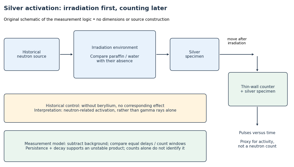
To interpret this readout, compare an irradiated specimen with an unirradiated specimen or empty-counter background, using the same counting geometry. Compare irradiation conditions at matched irradiation durations, delays and counting windows. These are requirements of the measurement model, rather than a claim that every such control is documented in the short October letter. Otherwise ordinary radioactive decay during transfer can imitate a change in activation. A persistent, decaying excess after irradiation supports an unstable product; neither a larger count nor a fitted half-life uniquely identifies an isotope.

In his 1938 Nobel lecture, Enrico Fermi distinguished single and superposed exponential decay curves and described chemical separation to identify their carriers. His slowing interpretation connected elastic collisions with enhanced capture. The lecture also described neutron capture resonances, so its account cannot support a universal rule that slower always means more reactive.^[ref]

The 1934 assignments of some uranium activities to elements beyond uranium were mistaken interpretations, not a discovery of nuclear fission. The published lecture's later footnote explicitly calls for reexamining the transuranic assignments after evidence of splitting. Distinguish that correction from the lecture as delivered.^[ref]

A neutrino label defined by the associated charged lepton in weak charged current production or detection. A produced flavour state can evolve through neutrino oscillation.

The mass of a neutrino mass eigenstate. A neutrino flavor need not have one definite mass; neutrino oscillation probes differences of squared masses.

The neutrino flavor associated with the tau lepton in the weak charged current. Its direct detection through interactions producing a tau lepton was announced by the DONUT experiment in 2000.^[ref]

The electron neutrino is the neutrino flavour associated with the electron in the weak charged current.

An atmospheric neutrino is produced in a cosmic-ray air shower, principally through decays of secondary mesons and muons. For example, a charged pion can produce a muon and a muon-flavor neutrino; the later muon decay produces additional electron- and muon-flavor neutrinos or antineutrinos.

The direction determines a broad range of propagation distances: downward events originate relatively nearby, whereas upward events can arrive through Earth from the opposite atmosphere. Comparing event distributions by direction and energy therefore tests flavor conversion over different baselines. The 1998 Super-Kamiokande analysis found a direction-dependent muon-neutrino deficit consistent with oscillations, using a large water detector to observe charged interaction products.^[ref] The incident spectrum and interaction probabilities remain part of the inference.

A Majorana neutrino is its own antiparticle. A corresponding mass term can violate conventional lepton number by two. Observing a wrong-helicity charged-current process is nevertheless suppressed by the very small neutrino mass relative to its energy, rather than having the ordinary charge-conjugate branching fraction.

A Boltzmann machine is a stochastic neural network that learns a probability distribution specified by pairwise energies. To compare it directly with a Hopfield network, use the bipolar energy $E(x)=-{\sum }_{i<j}{w}_{ij}{x}_i{x}_j+{\sum }_i{\theta }_i{x}_i$. Here $\beta >0$ controls the preference for low energy, and the partition function $Z={\sum }_x{e}^{-\beta E(x)}$ normalizes all states. In a computational model, $\beta$ is an algorithmic inverse temperature; interpreting it as $1/(k_{B}T)$ additionally requires physical energy units.

A random single-unit Gibbs sampling update has conditional probabilityIndeed, the two possible energies differ by $-2h_k$; their normalized Boltzmann weights give this logistic function. Random selection of one unit at a time satisfies detailed balance. For finite weights and finite positive $\beta$, all conditional probabilities lie strictly between zero and one, so the finite Markov chain can reach every state and can remain in place. Its unique stationary distribution is $p_{\beta }$. A short run need not yet sample that distribution accurately.

As $\beta \to \infty$, a nonzero field selects its sign, approaching asynchronous Hopfield energy descent. At zero field the stochastic rule remains a fair coin, whereas the deterministic convention above retains the old value. At finite inverse temperature, uphill moves permit exploration beyond one local minimum. Recall and learning are different operations: sampling changes the units at fixed weights; learning changes the weights to fit the training data.

An associative memory retrieves a stored pattern from a related cue. An incomplete cue supplies only some coordinates; a corrupted cue supplies some wrong coordinates. A Hopfield network implements retrieval by making intended patterns stable states with surrounding basins of attraction. This turns correction into a collective computation: no unit needs to know the entire desired answer. A cue outside the appropriate basin of attraction can retrieve another pattern or an unintended stable state.

For a periodic spin-one-half Heisenberg model $H=-(J/{\hslash }^2){\sum }_{n=1}^N{\mathbf{S}}_n\cdot {\mathbf{S}}_{n+1}$, $J>0$, the fully aligned state has $E_0=-NJ/4$. In its single-excitation subspace, let $|n⟩$ denote a down spin at site $n$ in an otherwise up background. Direct action of each bond givesThe normalized translation eigenstates are $|q⟩=N^{-1/2}{\sum }_n{e}^{iqna}|n⟩$, with $q=2\pi \ell /(Na)$ modulo $2\pi /a$. Their energy eigenvalues are $E_0+J[1-\cos (qa)]$. This is an exact one-magnon calculation, not a many-magnon harmonic approximation. Near $q=0$ the energy above $E_0$ is $J{a}^2{q}^2/2$.

The wavenumber restriction comes from requiring a periodic plane-wave coefficient pattern, equivalently requiring this vector to be an eigenvector of a one-site translation with eigenvalue $e^{-iqa}$. The identity $T^N=I$ alone imposes no restriction on a general state: it already holds throughout the ring Hilbert space. An arbitrary finite sum with coefficients $e^{iqna}$ still returns after $N$ translations, but need not be a one-site translation eigenstate unless $e^{iqNa}=1$.