Topics (384k) Articles (398k) Users (410) Discussions (242) Comments (383) Files (13k) New article

The simulation separates a stipulated physical distribution from measurement broadening. Its Cauchy distribution is only a convenient resonance-shaped input, not a complete quantum scattering model. Spatial resolution, magnetic field calibration, Multiple Coulomb scattering, stopping power and incorrect daughter identities all propagate into the measured invariant mass. Instrumental broadening must be understood before interpreting an observed width as a lifetime.
Selection also changes the shape. A momentum threshold can remove low-invariant mass pairs; a fit that fixes the candidate parent's mass would artificially concentrate that same mass and cannot supply an independent search distribution. Compare accepted simulated events with the input distribution, vary justified selection criteria, and check neighboring invariant mass intervals. A peak supported only by one untested selection is weaker evidence than a structure that survives calibration and background checks. The smooth background in the figure is a stipulated control component, not a claim that every physical background is smooth.
Take two stipulated oppositely charged daughters with equal rest mass and exactly opposite momenta of magnitude . Their total momentum is zero, soThis is a constructed event, not an identification of a historical particle. Boosting both four-momenta by along the first daughter's direction gives total energy and total momentum . Substitution recovers the same invariant mass, although the laboratory energy has increased.
The following independent simulation stipulates 700 signal combinations from a Cauchy distribution centered at with scale , truncated to , plus 2400 background combinations whose density decreases linearly across that interval. Each combination is converted to a back-to-back two-daughter event with . Independent isotropic directions are chosen, each Cartesian momentum component receives normal distribution noise with standard deviation , and invariant mass is reconstructed from the perturbed momenta. All inputs and counts are invented. No historical experimental points or fitted historical parameters appear.
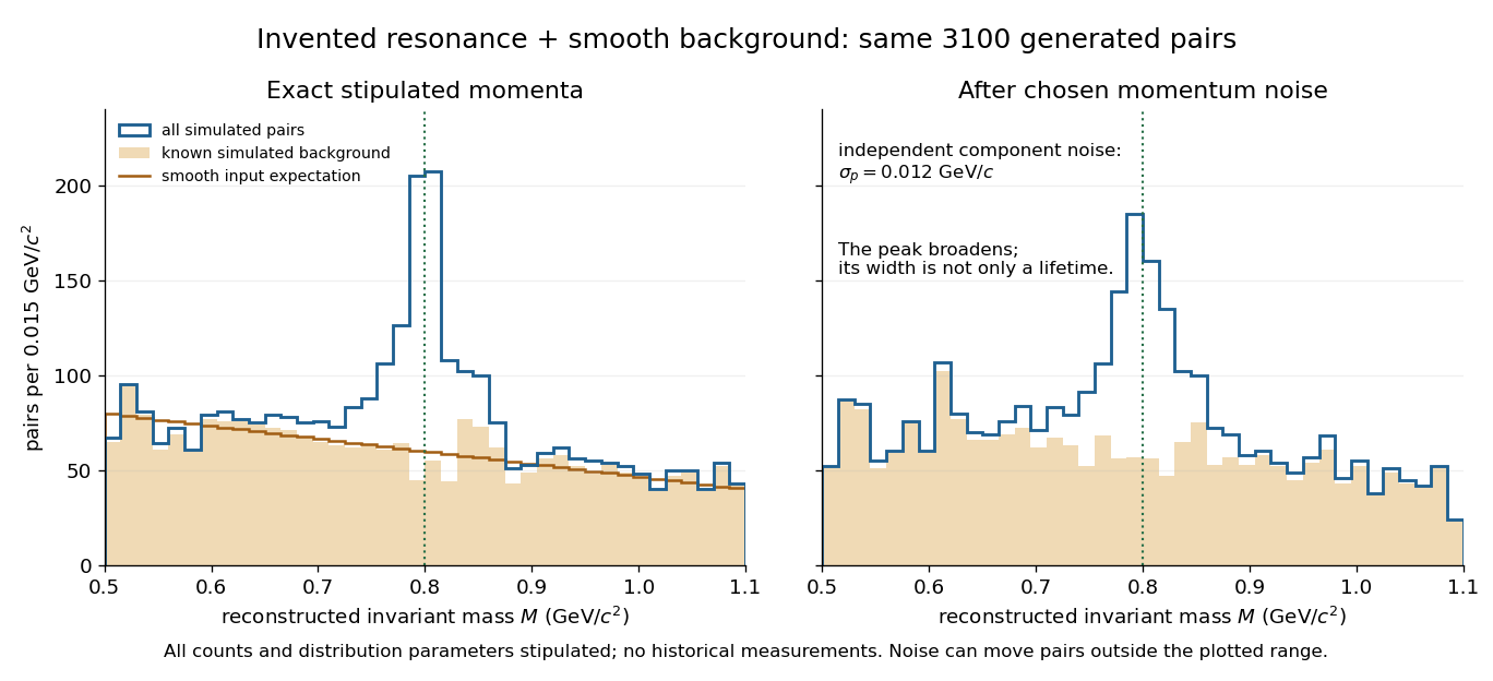
A stipulated resonance component produces an excess above a smooth simulated invariant-mass background
. Original simulation of two-daughter events, with invented counts, a truncated Cauchy signal and a linearly falling background. The two panels share the same generated events. The right panel adds chosen momentum noise before reconstructing invariant mass; this is not an experimental discovery plot. Details.For torque-free rotation, total angular momentum magnitude and rotational kinetic energy are conserved. Near rotation about principal axis three, eliminate from to obtain the displayed energy difference from . If is largest, it is a constrained energy minimum; if smallest, a maximum. Both extrema are stable in the conservative problem. An intermediate moment gives opposite signs in the quadratic form, a saddle and instability. Dissipation changes the fixed-energy argument and must not be silently added to torque-free motion.
A trigonometric substitution is integration by substitution using a trigonometric function to simplify an integrand, especially a square root. For example, , with and , changes to and to . The interval restriction fixes the sign of the square root. Similarly simplifies . The transformed integral must include the differential and, for a definite integral, the new limits.
A neutral isotropic atom with static electric polarizability in the field of a distant point charge has induced dipole and energy . Since ,The negative radial force is attractive for either sign of . Reversing reverses the induced dipole but not the energy or leading force. The factor accounts for the work of inducing the dipole; using the permanent-dipole energy without that work would double the answer. The approximation assumes weak fields, a slowly varying field across the atom and negligible electronic overlap.
A localized orbital with two electron spin states has energies , and . Its zero-temperature equilibrium occupation minimizes , where is the chemical potential. For repulsion , the occupation is successively as crosses and . For attraction , the singly occupied state is never the minimum: the occupation jumps from to at . Exactly at a crossing the ground-state occupation is not unique.
At positive temperature, its grand canonical partition function is , where . The expected value of the occupation follows by differentiating: . The factor two counts the two singly occupied microstates, not an additional pair state.
A function has an integrable singularity at a point if it becomes unbounded there but its absolute value has a finite improper integral over a sufficiently small surrounding interval, one-sided at an endpoint. The endpoint behavior of the arcsine distribution's probability density function is an example.
For a real matrix and a fixed vector , every vector in the image of a linear map defined by is orthogonal to exactly when . Indeed, . If this vanishes for every , choose to obtain . Equivalently each column of is orthogonal to . Requiring the statement only for nonzero changes nothing, since the zero input already has zero dot product. This is the orthogonal complement relation between the image of a linear map and the kernel of a linear map defined by its transpose.
A real charge at outside a spherical conductor of radius has the usual grounded-sphere image charge at . Adding a central image makes the total image charge zero, representing an isolated neutral conductor. The off-centre pair has zero potential on ; the central image therefore sets the constant conductor potential to . Its induced electric dipole moment is . Keeping the applied central field fixed gives . As , the external field becomes uniform near the sphere; its divergent constant potential can be removed without affecting the electric field.
Connect a resistor from the input source to the inverting input, a feedback resistor from output to that same input, and ground the non-inverting input. For ideal linear operation the inverting node is a virtual ground. Kirchhoff's current law gives , yielding the displayed voltage gain. The source sees input impedance , even though the amplifier input itself has infinite input impedance.
A diamond anvil cell compresses a sample between opposed diamond tips. The flat diamond anvil culets load a metal gasket whose hole holds the specimen and a pressure-transmitting medium. Transparent diamond admits excitation and returning fluorescence, enabling an internal ruby pressure sensor.[ref]
High Pressure X-Ray Crystallography With the Diamond Cell at NIST⁄NBS by Gasper J. Piermarini. Sections 2–3, Figures 1 and 5: anvils, optical path and gasket
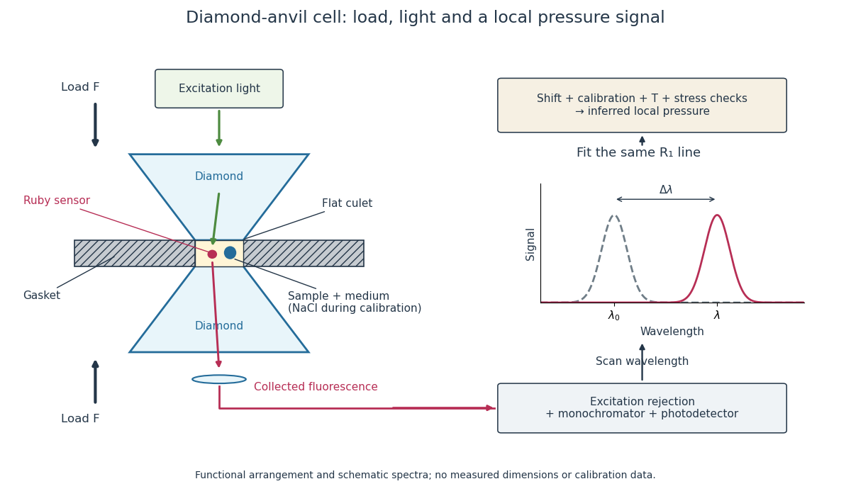
Diamond anvil cell: compression, optical access and internal ruby readout
. Original functional section, not a reconstruction or a scale drawing. The separate excitation and collection paths depict one possible arrangement. A monochromator and photodetector resolve the fluorescence emission spectrum; the inference uses a spectral line position rather than its brightness. The optional sodium chloride reference belongs to the calibration experiment, rather than to every subsequent sample measurement. Details.The functions in the drawing answer different questions. The drive applies force, the gasket confines the sample, the medium transmits stress, and the ruby pressure scale assigns a local pressure from an optical signal. A large drive reading cannot establish either the sample's pressure or the absence of deviatoric stress. Optical access also permits repeated readings without unloading the sample: a change during a long measurement can be detected rather than silently folded into a material-property curve.
Pressure calibration assigns pressure values to a sensor's output by comparison with a reference under specified conditions. It is not the same as making the output more finely resolved. A smooth electrical resistance curve can be repeatable yet have an incorrect pressure scale.
Bridgman used pressure-dependent electrical resistance of manganin and established fixed points, including a bismuth transition. He reported poorer accuracy above the better calibrated range.[ref]
General Survey of Certain Results in the Field of High-Pressure Physics by Percy Williams Bridgman. p. 56, pressure-measurement paragraph: manganin gauge, bismuth fixed point, and different accuracy estimates below and above 30000 kg/cm²
A fixed-point specimen and a property-measurement sample have distinct roles: one helps assign the scale, while the other is studied on that scale. The reference transition must itself have an assigned pressure at the relevant temperature. Agreement at a single point does not determine a nonlinear sensor response elsewhere. Comparing increasing and decreasing pressure checks hysteresis; returning to a reference checks drift. These are checks one can design from the measurement model, not additional historical controls asserted for the lecture's experiments.
With tension taken positive, hydrostatic stress is the stress tensor , where is the identity matrix. Every plane has the same compressive normal stress, and no tangential traction. More generally,where is deviatoric stress. Two samples can share the same mean pressure while experiencing different deviatoric stresses. A stationary liquid cannot sustain equilibrium shear stress; a solid transmitting medium can support it. Consequently, a load divided by surface area does not by itself establish hydrostatic sample conditions. A transmitting medium's state at the actual pressure and temperature, and contact between sample and walls, matter.
Bridgman's Figure 4 compares mild steel fractured in tension at atmospheric pressure with steel stretched further in a liquid at .[ref]
General Survey of Certain Results in the Field of High-Pressure Physics by Percy Williams Bridgman. p. 56, Figure 4 caption: atmospheric-pressure tensile fracture versus greater reduction of area in pressurized liquid; historical kg/cm² rendered explicitly as force per area
The imposed tension remains a directional load: the experiment combines confinement with deformation, rather than measuring a hydrostatic stress alone. Its comparison motivates recording the loading path and the surrounding medium as well as pressure; it does not establish a universal fracture threshold for all steels.In a functional model, a driven piston reduces the chamber's volume. A surrounding cylinder carries the wall stress; a deformable packing or gasket closes a potential leak path around a moving or removable closure. A sample and a separate pressure sensor occupy the chamber. A transmitting liquid can load the sample on all sides; the sensor's signal passes to an external readout. This is a division of experimental functions, not a scale reconstruction of one historical machine.
For a slowly moving frictionless drive piston of effective surface area , external pressure and inward applied force , Newton's second law at mechanical balance givesThus on a stipulated effective surface area corresponds ideally to of differential pressure. These are illustrative numbers, not apparatus specifications. The effective surface area is the one associated with the pressure difference, not necessarily an external ram's visible cross section. With resisting friction during inward motion, the balance becomes . During outward motion the sign of the friction contribution reverses. An applied-load reading can therefore show hysteresis even when the chamber's actual pressure is well defined.
A resistance pressure gauge instead supplies an internal signal. In a generic electrical readout, measure an electric potential difference with a known electric current and use Ohm's law to infer electrical resistance . This describes a possible readout principle; the lecture passage cited below identifies the sensor material and calibration landmarks without specifying this wiring.
In four spacetime dimensions a massless vector has two physical polarizations, while a Proca field has three. Before rearrangement, the electroweak sector has four vector fields and four real Higgs doublet components, hence twelve propagating degrees of freedom. In the broken description, W bosons of both charges and the Z boson contribute nine, the photon contributes two, and the radial Higgs boson contributes one. The three angular scalar components supply the three additional longitudinal polarizations. Gauge components and constraint variables are excluded from both counts. The gluon sector is unaffected.
In their 1964 paper, François Englert and Robert Brout showed that gauge bosons associated with generators that rotate the chosen vacuum acquire masses while gauge invariance is maintained. Their discussion included both scalar and fermionic models.[ref]
Broken Symmetry and the Mass of Gauge Vector Mesons by François Englert and Robert Brout. pp. 321–323, especially Eq. (6)
Independently, Peter Higgs exhibited a massive vector and a surviving massive scalar field by linearizing a simple gauge theory. His paper explicitly distinguishes this classical calculation from a proof for the full quantized theory. These 1964 mechanisms supplied an ingredient for the later electroweak interaction, rather than the complete Standard Model.[ref]
Broken Symmetries and the Masses of Gauge Bosons by Peter Higgs. p. 508, Eqs. (2b)–(4); p. 509, note 4
The ATLAS experiment and CMS experiment searched proton-proton collisions at the Large Hadron Collider at collision energies of and . The ATLAS experiment used silicon tracking, a solenoid, liquid-argon electromagnetic calorimeters and an external muon spectrometer. Its July 2012 paper reported a combined local statistical significance of standard deviations near ; this paper result is distinct from the initial 4 July announcement.[ref]
The CMS experiment used silicon tracking in a solenoid, lead-tungstate electromagnetic calorimeters and external muon chambers. Electrons combine tracks and particle showers; muons combine tracking and chamber hits; photons supply shower energies and directions. Selected and candidates, with , yielded invariant mass peaks. It checked lepton efficiencies with Z boson decays, estimated fake-lepton backgrounds from control samples with relaxed identification, and fitted the smooth diphoton background from data. Its combined local statistical significance was standard deviations near .[ref]
The ATLAS experiment compared signal-plus-background and background-only hypotheses with a profile likelihood, accounting for systematic uncertainties and correlations between decay channels. Diphoton and four-lepton candidates gave precise invariant masses; decays supplied additional evidence with poorer mass reconstruction because of escaping neutrinos. A local p-value concerns one specified mass; scanning masses requires a look-elsewhere effect correction.[ref]
Two-photon decay excludes spin one under the usual assumptions, but does not prove spin zero. A mass peak does not determine every Higgs boson coupling. Production rates, branching fractions and angular correlations require additional tests.[ref]
With the conventional electroweak vacuum value , the electron Yukawa coupling is and the physical Higgs-electron vertex coefficient is . Direct s-channel Higgs production in electron-positron annihilation is consequently very small away from a compensating resonance enhancement. This suppression belongs to the coupling at the initial vertex, not to a prohibition on the Higgs boson coupling to W bosons.
Consider an original model of a cold section enclosing a throttle and collecting region, with the precooling heat exchanger outside its boundary. The inlet has mass flow rate and specific enthalpy . The outlets are equilibrium liquid and vapor at one fixed pressure, with specific enthalpies and . Let be the outlet liquid mass fraction, and let be incoming unwanted heat per unit incoming mass. Assume steady flow, no shaft work, and negligible bulk kinetic energy and gravitational potential energy changes. The steady-flow energy balance givesHere is the latent heat per unit mass at the chosen outlet pressure. The mass flow rates of the outlets are and . The formula describes a flowing cold section; a filling vessel with appreciable energy or mass accumulation requires storage terms.
For a deliberately dimensionless example, choosePer unit incoming mass, one quarter leaves as liquid and three quarters as vapor. With zero incoming heat, the same inlet would give . Increasing to reduces to , and reaches the no-liquid boundary. These are chosen model values, not helium property data or a historical yield. In normalized enthalpy units with and , conservation checks directly: .
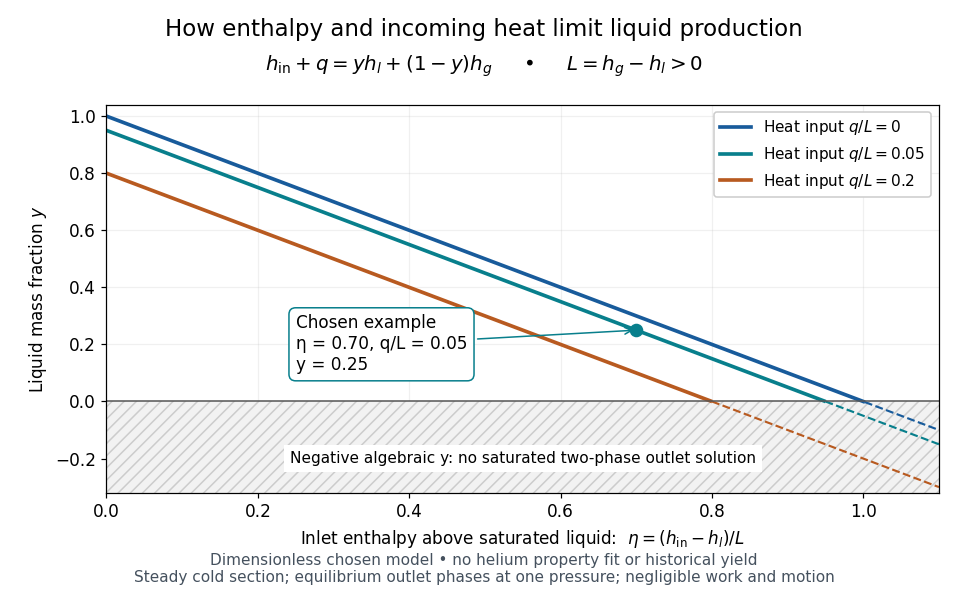
An original normalized liquefaction enthalpy budget
. Each solid segment satisfies the stipulated equilibrium two-outlet model. Dashed negative continuations are algebra only: they do not describe a negative liquid mass fraction. No helium properties or experimental measurements were fitted. Source. Details.The admissible interval is , or . Outside it, the assumed equilibrium two-phase outlet fails: an enthalpy above requires a hotter single-vapor outlet under these assumptions, rather than a negative amount of liquid. Below , a colder liquid or a different thermodynamic phase must be considered. The balance does not predict its own outlet pressure, temperature or helium property functions.
At fixed outlet pressure, hence fixed , the derivatives are and . Lowering inlet specific enthalpy by regeneration and reducing incoming heat therefore buy the same increase in liquid mass fraction per unit energy per unit mass in this model. Adding any constant to all three specific enthalpies leaves unchanged. This independence of the arbitrary enthalpy reference makes the balance useful even when property tables choose different zero points.
On 10 July 1908, Heike Kamerlingh Onnes's Leiden laboratory circulated purified helium through liquid air and evaporatively cooled liquid-hydrogen precooling, a regenerative heat exchanger, and an expansion valve. Returning helium cooled incoming helium; liquid collected in a transparent vacuum vessel. Reflected light revealed its liquid meniscus, crossed by thermocouple wires. Subsequent mass density and spectroscopy checks tested contamination.[ref]
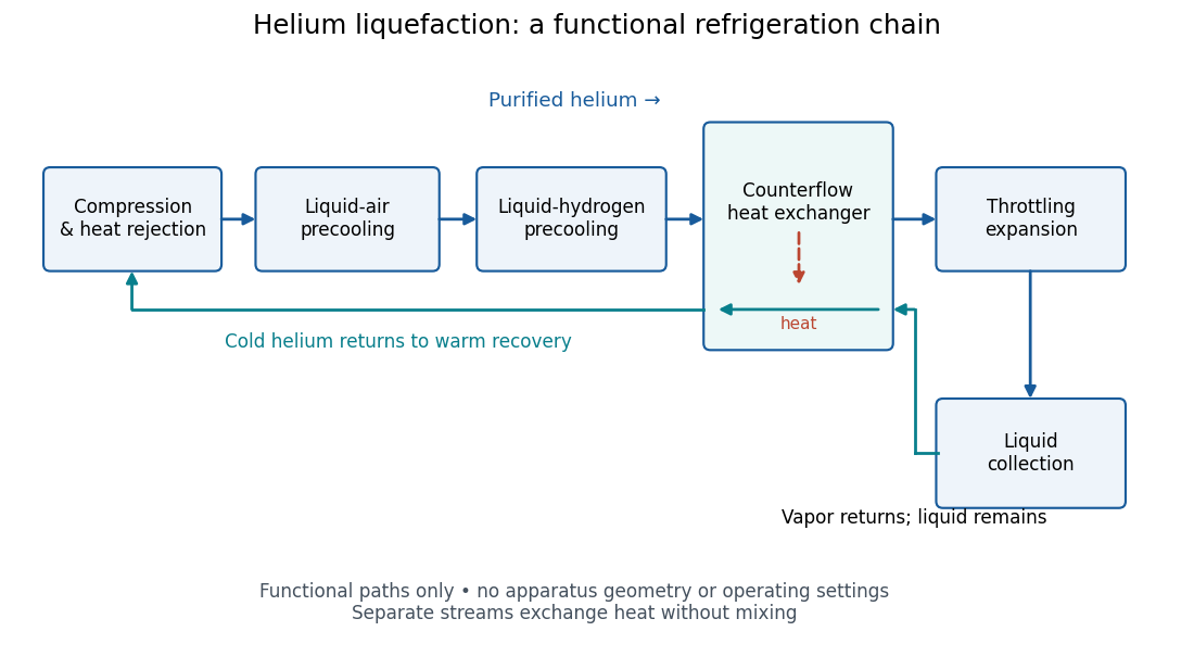
Functional stages of helium liquefaction
. Original functional diagram of the reported sequence. Arrows show stream direction and heat transfer; positions do not represent the apparatus geometry. Compression and heat rejection close the refrigeration cycle. Source. Details.A constant-volume helium gas thermometer below the valve supplied the temperature indication. An oxygen boiling reference check disagreed with its expected reading; the real gas correction to thermodynamic temperature remained provisional. A temperature plateau suggested immersion before the liquid meniscus was recognized.[ref]
The Liquefaction of Helium by Heike Kamerlingh Onnes. §4, pp. 180–181; §§5–6, pp. 183–184
The measurement principles separate two questions. A visible liquid meniscus establishes an interface; a gas thermometer estimates temperature through an equation of state. A stationary temperature trace can also result from a steady state without phase coexistence, so it cannot replace the interface observation. Conversely, seeing a liquid does not calibrate a thermometer. Thermometer calibration, the gas thermometer dead-space correction, departures from the ideal gas law and incomplete thermal equilibrium all matter when assigning an absolute temperature. A check far from the intended measurement range tests the instrument but does not by itself bound every low-temperature error.
Pinned article: Introduction to the OurBigBook Project
Welcome to the OurBigBook Project! Our goal is to create the perfect publishing platform for STEM subjects, and get university-level students to write the best free STEM tutorials ever.
Everyone is welcome to create an account and play with the site: ourbigbook.com/go/register. We belive that students themselves can write amazing tutorials, but teachers are welcome too. You can write about anything you want, it doesn't have to be STEM or even educational. Silly test content is very welcome and you won't be penalized in any way. Just keep it legal!
Intro to OurBigBook
. Source. We have two killer features:
- topics: topics group articles by different users with the same title, e.g. here is the topic for the "Fundamental Theorem of Calculus" ourbigbook.com/go/topic/fundamental-theorem-of-calculusArticles of different users are sorted by upvote within each article page. This feature is a bit like:
- a Wikipedia where each user can have their own version of each article
- a Q&A website like Stack Overflow, where multiple people can give their views on a given topic, and the best ones are sorted by upvote. Except you don't need to wait for someone to ask first, and any topic goes, no matter how narrow or broad
This feature makes it possible for readers to find better explanations of any topic created by other writers. And it allows writers to create an explanation in a place that readers might actually find it.
Figure 1. Screenshot of the "Derivative" topic page. View it live at: ourbigbook.com/go/topic/derivativeVideo 2. OurBigBook Web topics demo. Source. - local editing: you can store all your personal knowledge base content locally in a plaintext markup format that can be edited locally and published either:This way you can be sure that even if OurBigBook.com were to go down one day (which we have no plans to do as it is quite cheap to host!), your content will still be perfectly readable as a static site.
- to OurBigBook.com to get awesome multi-user features like topics and likes
- as HTML files to a static website, which you can host yourself for free on many external providers like GitHub Pages, and remain in full control

Figure 2. You can publish local OurBigBook lightweight markup files to either OurBigBook.com or as a static website.
Figure 3. Visual Studio Code extension installation.
Figure 5. . You can also edit articles on the Web editor without installing anything locally. Video 3. Edit locally and publish demo. Source. This shows editing OurBigBook Markup and publishing it using the Visual Studio Code extension. 
- Infinitely deep tables of contents:




All our software is open source and hosted at: github.com/ourbigbook/ourbigbook
Further documentation can be found at: docs.ourbigbook.com
Feel free to reach our to us for any help or suggestions: docs.ourbigbook.com/#contact