Use the independent spin-one-half two-level system with fixed $N$ distinguishable sites and Hamiltonian levels $E_{\pm }=\pm \mu B$, where $\mu >0$ is the magnitude of the field-axis magnetic moment and $B>0$ is a uniform externally controlled magnetic field. Assume positive temperature, no interactions between sites, and no appreciable lattice or load entropy. The two levels differ by $2\mu B$. With inverse temperature $\beta$, the canonical ensemble gives the one-site and total partition functionsHere the minus subscript denotes the lower energy $-\mu B$. Factorization of the partition function requires additive energy and independent sites; there is no particle-exchange factor $N!$ for these fixed distinguishable sites.

Differentiate the partition function, holding $B$ fixed when differentiating with respect to $\beta$. The internal energy, Helmholtz free energy, total field-axis magnetic moment $m$, and magnetic entropy areThe extensive moment $m$ is distinct from magnetization, the moment per unit volume. Direct substitution of $p_{\pm }$ into the Gibbs entropy gives the same $s(x)$ independently of the free-energy derivative.

At fixed $B$, the magnetic heat capacity isStrict decrease makes $s$ invertible on $x>0$. Constant magnetic entropy therefore fixes $x$, not $B$ or $T$ separately:The partition function may be used to label these equilibrium states even though the isolated cooling leg has no external heat bath. Actual thermalization of the lattice and load additionally requires a sufficiently fast spin-lattice relaxation; perfectly uncoupled spins by themselves cannot refrigerate an attached object.

The limiting cases are instructive. For $x\ll 1$, $s(x)=\ln 2-x^2/2+O(x^4)$, $m\simeq N{\mu }^{2}B/(k_{B}T)$, and $C_{B,\mathrm{mag}}\simeq N{k}_B{x}^2$. The moment response reproduces Curie's law. For $x\gg 1$, $s(x)\simeq (1+2x)e^{-2x}$ and the upper-state occupation is exponentially small. Taking $B\to 0$ at fixed $T>0$ gives $s\to \ln 2$; taking $T\to 0$ at fixed $B>0$ gives $s\to 0$. The origin has a path-dependent limit. Extrapolating a line of constant $x$ to $B=T=0$ does not construct a usable zero-temperature state or prove that a real material retains independent degenerate spins there.

A magnetic domain wall separates differently oriented magnetic domains. Its motion changes their volumes and average magnetization. It is a magnetic domain wall.

An original two-magnetic domain model makes the collective change explicit. Suppose opposite regions have magnetizations $+M_s$ and $-M_s$ along the measuring axis, where $M_s$ is the local saturation magnetization. If a magnetic domain wall sweeps volume $\Delta V$ from the negative region into the positive one, in a specimen of fixed volume $V$, thenThe factor two comes from replacing $-M_s$ by $+M_s$. The local magnitude $M_s$ stays fixed while the average magnetization changes; the event size depends on the swept volume, rather than a universal single-spin increment.

Calorimeter addenda are the participating heat capacity of everything in the measured thermal assembly except the sample: platform, heater, thermometer, mounting material and the effective part of the leads. They depend on temperature and assembly details. Calorimeter calibration can determine them using an empty platform or a reference sample. Subtract $C_a(T)$ from the loaded assembly at matching temperature and applied magnetic field; replacing it with a constant can imitate a sample anomaly.

For a charge $q$ of mass $m$ bound by spring constant $k=m{\omega }_0^2$, the undamped equation $m\ddot{x}+kx=q{E}_0{e}^{-i\omega t}$ has complex amplitude $x_0=q{E}_0/[m({\omega }_0^2-{\omega }^2)]$. The induced electric dipole moment is $p_0=q{x}_0$. Averaged electric dipole radiation power, divided by incident light intensity, givesThe Rayleigh scattering limit $\omega \ll {\omega }_0$ gives $\sigma \sim {\sigma }_T(\omega /{\omega }_0{)}^4$, proportional to ${\lambda }^{-4}$. For ${\omega }_0\ll \omega \ll m{c}^2/\hslash$, the charge behaves as free and the Thomson cross-section is recovered. At resonance the undamped steady-state formula is invalid; a finite damping mechanism or radiation reaction must be included. The formula describes independent weakly driven scatterers, not arbitrary coherent scattering from an extended medium.

For $\ddot{z}+2\gamma \dot{z}+{\omega }_0^{2}z=(q{E}_0/m)\cos \omega t$, the $e^{i\omega t}$ convention gives complex displacement amplitude $\tilde{z}=(q{E}_0/m)/({\omega }_0^2-{\omega }^2+2i\gamma \omega )$. If the real amplitude is defined nonnegative, the phase is $-\delta$ for $q>0$ but $\pi -\delta$ for $q<0$, where $\delta =atan2(2\gamma \omega ,{\omega }_0^2-{\omega }^2)$. An electron's low-frequency displacement is opposite to the electric field; its high-frequency displacement is in phase. The induced electric dipole moment $qz$ instead has phase $-\delta$ for either sign of charge. A signed amplitude can absorb the extra $\pi$, but that convention must be stated.

An optical oscillator strength is a dimensionless weight assigned to an optical resonance. In an independent-resonance Lorentz oscillator model using a reference electron mass $m_e$ and a specified participating number density $n$,Its normalization must be stated: assigning one unit of total strength per participating electron means ${\sum }_j{f}_j=1$. A one-resonance approximation with $f_1=1$ represents the whole chosen electron population, rather than asserting that the first allowed interband transition carries all optical strength. The smallest band gap therefore need not equal the fitted resonance energy.

The Lenard cathode-ray window experiment lets cathode rays leave a gas-discharge tube through a thin aluminium foil while preserving the tube's vacuum. This separates production from propagation.

Philipp Lenard's lecture, delivered on 28 May 1906, describes sealing a small hole in a metal plate with aluminium foil. Luminous phosphor grains first rested on the window, then glowed above it in air. His improved tube separated production and observation chambers; coated paper served as a fluorescent screen. An aperture revealed spreading beyond a narrow straight beam. Evacuating the observation chamber reduced spreading and attenuation without interrupting production. Interposed layers and stepped foil stacks gave shadow comparisons; approximate scaling with mass had exceptions.^[ref]

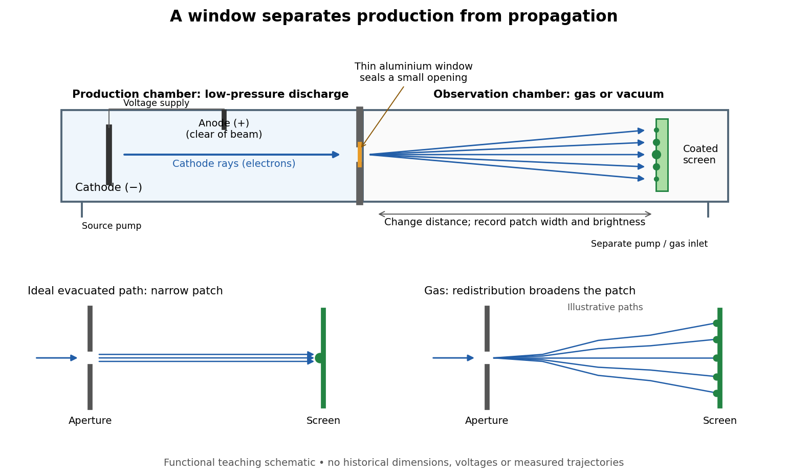
The experimental advantage is unusually clean: reducing the gas content in the observation chamber tests whether gas is needed to carry the cathode rays, while retaining the conditions needed to generate them. The window is a boundary that transmits some electrons while confining the source environment. A spot outside establishes a transmitted effect; the aperture and changed observation environment provide additional ways to distinguish propagation from the source's behavior. This logic is useful whenever a complicated source would otherwise be changed by the very intervention intended to test the emitted beam.

Several inferences require care. A darker fluorescent screen can mean fewer arriving electrons, less deposited energy per electron, or redistribution by electron scattering beyond the observed area. A visible endpoint depends on the screen's sensitivity and background. It is not an intrinsic electron range independent of initial kinetic energy, gas density, and observation geometry. For a modern comparison, measure a reference at fixed source conditions, use background subtraction, and compare the whole luminous patch as well as a small central region. A wider collection area tests redistribution; changing source-to-screen separation also changes collection geometry. These are proposed controls for interpreting a readout, not additional historical observations attributed to Lenard.

Nor is fluorescence a unique signature of cathode rays: X-rays can also excite it. Lenard notes that a later tube could transmit both, and that slow cathode rays failed to pass its window.^[ref] In modern terms, cathode rays are electrons carrying negative electric charge, whereas X-rays are photons with zero electric charge. Magnetic bending of the incident electrons, interpreted through the Lorentz force, supplies a discrimination that brightness alone cannot. Passage through foil alone determines neither the sign of electric charge nor its magnitude, and it does not measure charge-to-mass ratio. The separate Thomson charge-to-mass experiment explains that inference. Even a measured charge-to-mass ratio needs an independent electric charge measurement to determine mass.

The Thomson charge-to-mass experiment infers the magnitude of an electron's charge-to-mass ratio by combining electric and magnetic deflection of cathode rays. The central idea is to determine speed separately from magnetic curvature: a known speed turns the observed gyroradius into a measurement of $e/m$.

In 1897, J. J. Thomson used two grounded slits in an evacuated glass tube, then aluminium plates $5\mathrm{cm}$ long, $2\mathrm{cm}$ wide and $1.5\mathrm{cm}$ apart. A battery supplied their electric potential difference. Deflected cathode rays produced a phosphorescence patch on the glass; an external scale and movable luminous pointer recorded its position in darkness. Greater evacuation reduced gas electrical conductivity that screened the electric field; reversing plate polarity reversed deflection. External coils supplied the magnetic field, calibrated by induction against larger coils. He adjusted equal electric and magnetic deflections. ^[ref]

His comparison included air, hydrogen, carbon dioxide, and aluminium versus platinum cathodes, supporting a common carrier. He explicitly noted uncorrected magnetic bending outside the plates. His tables give $m/e$, the reciprocal of the magnitude used here. The inferred ratio alone could not separate electric charge from mass. ^[ref]

To connect this readout with the Lorentz force, derive a simple nonrelativistic model in modern SI notation. Let the uniform deflecting region have length $\ell$, followed by a field-free drift of length $L$. Assume a narrow speed distribution, small deflection angles, negligible collisions, and matching electric and magnetic field profiles. For an electron with speed $v$, the electric acceleration has magnitude $eE/m$, the transit time is approximately $\ell /v$, and the subsequent drift adds exit transverse velocity times $L/v$. Thus the displacement magnitudes measured separately with only electric field or only magnetic field areThe electric expression follows from constant transverse acceleration; the magnetic expression uses its small-deflection approximation. Equal displacement magnitudes then giveThis is an ideal derivation of the comparison principle, not a numerical reanalysis of the historical tube. Different exterior magnetic field profiles invalidate cancellation of the common geometrical factor. The comparison determines $e/m$ through deflection and the known apparatus dimensions; it does not require a downstream semicircle.

For a second, deliberately different teaching geometry, combine a velocity selector with a separate region containing only a uniform magnetic field $B_a$ perpendicular to the selected velocity. Here $B_s$ belongs to the velocity selector, while $B_a$ belongs to the analyzer: they need not be equal. The magnetic Lorentz force supplies the centripetal acceleration, soIf the analyzer turns the beam through a semicircle before it hits a screen in the entry plane, the separation $D$ between entrance and impact is the diameter: $r=D/2$. For a shorter observed arc, the screen displacement is not generally a radius; fit the appropriate circle geometry. This two-stage velocity selector and curvature apparatus is an original ideal teaching model, not a claim that Thomson's Fig. 2 used a separate selector and semicircular analyzer.

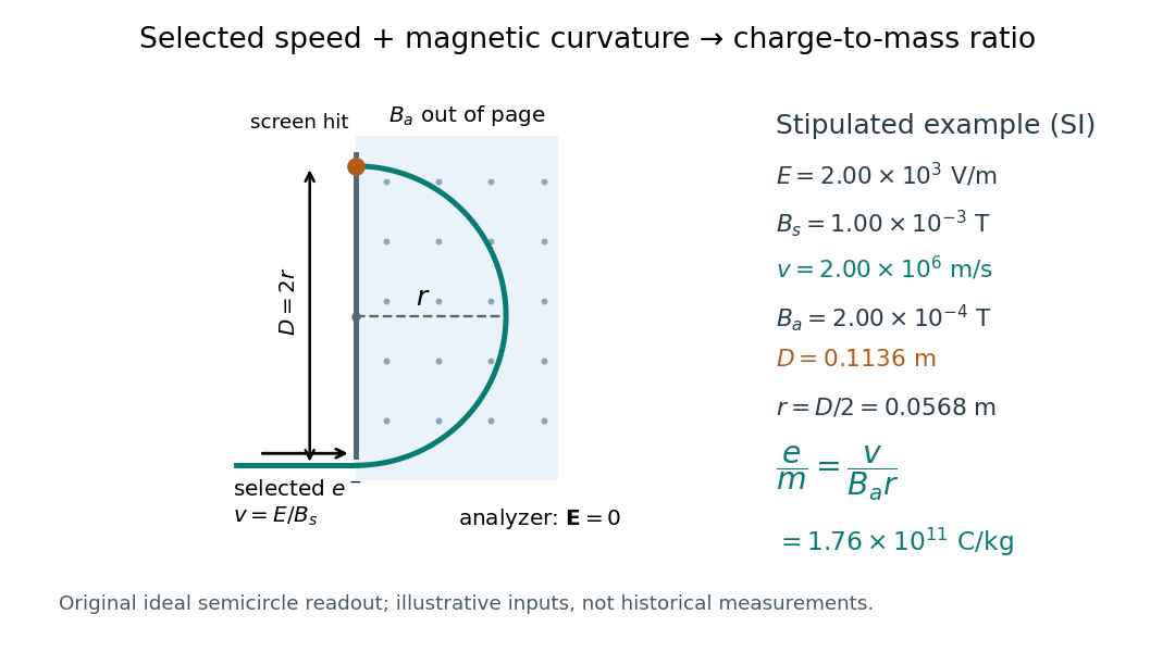
For a worked example, stipulate $E=2.00\times 10^3\mathrm{V}{\mathrm{m}}^{-1}$, $B_s=1.00\times 10^{-3}\mathrm{T}$, $B_a=2.00\times 10^{-4}\mathrm{T}$, and $D=0.1136\mathrm{m}$. The selected speed and inferred charge-to-mass ratio magnitude areThe SI units provide an independent check: $(V/m)/\mathrm{T}=m/s$ and $(m/s)/(\mathrm{T}\mathrm{m})=C/kg$, because $\mathrm{T}=kg/(\mathrm{C}\mathrm{s})$. The charge-to-mass ratio of the electron is negative; this calculation gives its magnitude. The bending direction gives the sign of the electric charge once the magnetic field direction is known. Scaling both $e$ and $m$ by the same positive factor preserves every displayed trajectory, so an independent electric charge measurement is required to determine mass separately.

The curvature formula assumes nonrelativistic momentum $p=mv$. At higher speeds, the relativistic cyclotron orbit gives $p=\gamma mv=e{B}_{a}r$, hence $e/m=\gamma v/(B_{a}r)$, where $\gamma$ is the Lorentz factor; the ideal straight-through selection $v=E/B_s$ still follows from vanishing Lorentz force. The stipulated speed is about $0.0067$ times the speed of light, making $\gamma -1$ about $2.2\times 10^{-5}$. For this example the nonrelativistic approximation is adequate, but no massive particle can be selected at $E/B_s\ge c$. Finite slit widths, collisions with residual gas, uncertain magnetic field calibration, and fields outside the ideal boundaries limit a real inference; repeat at several selected speeds and analyzer strengths to test consistency of $e/m$ rather than trusting one spot position.

A velocity selector uses perpendicular electric field and magnetic field to transmit a narrow range of speeds along a chosen beam direction. Assume uniform static electric field $\mathbf{E}=E\hat{\mathbf{y}}$ and magnetic field ${\mathbf{B}}_s=B_s\hat{\mathbf{z}}$, with $E,B_s>0$, and an incident velocity $\mathbf{v}=v\hat{\mathbf{x}}$. The cross product gives $\mathbf{v}\times {\mathbf{B}}_s=-v{B}_s\hat{\mathbf{y}}$, so the transverse Lorentz force isFor an electron, the electric force points downward and the magnetic force upward. A faster electron initially bends upward; a slower one initially bends downward. At the selected speed, both forces cancel along the whole straight trajectory. The cancellation is independent of mass and nonzero electric charge; it selects velocity, not a particular charge-to-mass ratio. A component of velocity parallel to the magnetic field is not constrained by the cancellation, so the incident beam must also have its direction restricted.

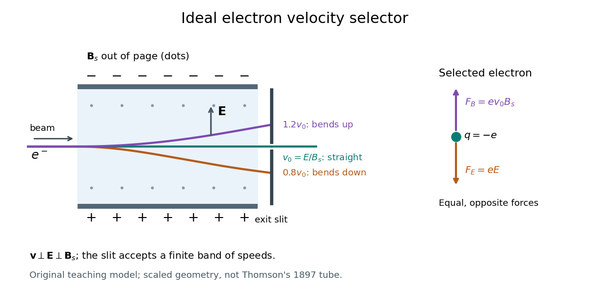
A real exit slit accepts a finite range of speeds and incident directions. A zero displacement at one screen alone does not establish zero force throughout the path: a curved trajectory could return to that screen position. The ideal velocity selector interpretation requires a straight aligned beam, known overlapping electric field and magnetic field, and sufficiently narrow entrance and exit slits. Its useful role in the Thomson charge-to-mass experiment teaching model is to supply speed independently of the subsequent magnetic bending.

The charge-to-mass ratio is a body's electric charge $q$ divided by its mass $m$. Its SI unit is the coulomb per kilogram, $\mathrm{C}\mathrm{k}{\mathrm{g}}^{-1}$. In a prescribed electric field and magnetic field, nonrelativistic acceleration depends on $q/m$ through the Lorentz force. Two bodies with the same initial position, velocity, and charge-to-mass ratio therefore have the same trajectory in this ideal model. For an electron, write $q=-e$ with $e>0$ the elementary charge: $q/m=-e/m$, whereas the positive number $e/m$ is the magnitude of the charge-to-mass ratio.

Magnetic rigidity measures the resistance of a charged particle's momentum to bending by a magnetic field. The relativistic cyclotron orbit gives $p_{\perp }=|q|Br$, where $r$ is the transverse gyroradius. For motion perpendicular to a uniform magnetic field, $p_{\perp }=p$ is the whole momentum. A measured magnetic rigidity fixes momentum per magnitude of electric charge; it does not by itself fix mass, kinetic energy, or the sign of the electric charge. This distinction makes the Anderson positron track experiment an especially revealing application of the Lorentz force.

For a free massless real scalar field with wave speed set to one and metric $(+,-)$, define $\mathcal{E}=({\varphi }_t^2+{\varphi }_x^2)/2$ and $p=-{\varphi }_t{\varphi }_x$. Its symmetric stress-energy tensor is $T^{\mu \nu }=\left(\begin{array}{cc}\mathcal{E}& p\\ p& \mathcal{E}\end{array}\right)$. The Lorentz current has density $tp-x\mathcal{E}$ and flux $t\mathcal{E}-xp$. Its conserved charge is the displayed expression when boundary flux vanishes. In one spatial dimension it generates boosts, not spatial rotations; there is no independent purely spatial angular-momentum component. Its conservation says that the center of energy moves uniformly. This is a symmetry of the wave-field model and need not survive boundaries or additional material effects.

For an eigenvector normalized by ${\sum }_{n=1}^N|{\psi }_n{|}^2=1$, the participation ratio in its site basis isIt estimates how many sites carry appreciable probability. Equal weight on $K$ sites and zero elsewhere gives $P=K$, irrespective of their wave phases. A single occupied site gives $P=1$; uniform probability on all sites gives $P=N$. These are exact constructed examples, not claims about particular Hamiltonian operators.

To prove the bounds, write $p_n=|{\psi }_n{|}^2$. Since $0\le p_n\le 1$, ${\sum }_n{p}_n^2\le {\sum }_n{p}_n=1$, giving $P\ge 1$. The Cauchy-Schwarz inequality gives $1=({\sum }_n{p}_n{)}^2\le N{\sum }_n{p}_n^2$, giving $P\le N$. Thus the measure has useful limits without assuming an exponential shape. Comparing $P$ as $N$ increases helps distinguish a state filling the sample from one occupying a fixed region, provided energy selection and disorder statistics are controlled.

The localization length $\xi$ measures the decay scale of a localized eigenstate's wave amplitude envelope. Here $a$ is the site spacing and $n_0$ its centre. With this amplitude convention, probability decays on half that scale:Individual random tails fluctuate; this notation describes their typical envelope, not exact equality at every site. A localization length much greater than a finite sample's length makes a state look extended inside that sample. The participation ratio below is an effective site count, not an independent fitted value of $\xi$.

An exponential decay rate $R=R_0{e}^{-t/\tau }$ becomes a straight line in $x=t$ and $y=\ln (R/R_{\ast })$, where $R_{\ast }$ is a fixed reference rate. Constant small fractional rate errors become approximately constant vertical errors $s\simeq {\sigma }_R/R$ by propagation of uncertainty. With independent Gaussian log-rate errors, linear least squares gives $\hat{m}=S_{xy}/S_{xx}$ and $\hat{c}=\bar{y}-\hat{m}\bar{x}$.

The covariance matrix is obtained by applying the variance rules to these linear estimators:Transforming back gives $\hat{\tau }=-1/\hat{m}$, ${\sigma }_{\tau }\simeq {\sigma }_m/{\hat{m}}^2$, ${\hat{R}}_0=R_{\ast }{e}^{\hat{c}}$ and ${\sigma }_{R_0}\simeq {\hat{R}}_0{\sigma }_c$. If a candidate lifetime fixes the slope $m_a$, the intercept must be refitted as $c_a=\bar{y}-m_a\bar{x}$. The profiled objective obeysThis follows by separating the centred slope residual from the unrestricted regression residual, whose inner product with the design columns is zero by the normal equations for linear least squares. Known supplied measurement errors are not rescaled by the observed reduced chi-squared. This log-error model is an approximation for proportional errors, not an exact replacement for every raw-count likelihood.

The linear attenuation coefficient divided by the material mass density.

The emitted optical power divided by electrical input power. For the bare-device calculation in light-emitting diode efficiency, $P_{\mathrm{elec}}=I{V}_f$; a complete lamp also consumes power in its driver. Luminous efficacy, measured in lumens per watt, additionally weights the spectrum by human visual sensitivity and is a different quantity.

The fraction of internally emitted photons that escape a light-emitting diode across the specified optical boundary. Collection by a particular detector adds another factor unless the measurement accounts for all escaping light.

The rate of escaping photons divided by the electrical pair-supply rate $I/q$ in a light-emitting diode. This counts photons rather than comparing optical and electrical power.

For the convention used in light-emitting diode efficiency, the internally generated photon rate divided by the rate of electron and electron hole pairs reaching the emitting layer. Its denominator must be stated when comparing measurements.