Topics (384k) Articles (398k) Users (410) Discussions (242) Comments (383) Files (13k) New article
The simplest Pease polynya model balances offshore ice export at speed against production of new ice at thickness rate within an open strip of width . Newly formed ice is collected into an edge of prescribed thickness , with negligible residence time. Per unit coastline length, conservation gives . For constant positive parameters,Thus the equilibrium width is and the relaxation time is . If warming reduces while stay fixed, both increase. With the positive-freezing equilibrium ceases to apply. Finite frazil ice residence, variable atmospheric forcing and alongshore transport require extensions of the model.
This reduced polynya model describes a wind-driven, nearly uniform surface layer containing dilute frazil ice. Let be distance from the opening, the layer depth, its horizontal speed, and its ice volume fraction. Use reference liquid mass density except in buoyancy, where is the liquid-minus-ice mass density difference. Let be the uniform wind shear stress and the atmospheric cooling heat flux divided by .
For a linear liquidus , far-field salinity , specific heat capacity and specific latent heat , define , and . The extra sensible term in accounts for the cooling associated with salt enrichment. The chosen depth-averaged momentum, ice-production and buoyancy balances areTheir numerical coefficients belong to this particular layer closure. The first two give and . Seeking a similarity solution with gives ; substitution into the third balance yieldsThus layer depth, speed and retained ice fraction all grow as . The increasing eventually violates the dilute approximation. If crystals are exported out of the layer, their enthalpy and ice-volume flux must be included through the frazil export enthalpy balance; retained fraction is not automatically total production.
There is a sequence of complex polynomials converging pointwise on the whole plane to the sign of the imaginary part, with value zero on the real axis. For each , take the compact union of the upper rectangle , its lower reflection and the real segment . Its complement is connected. The function equal to one, minus one and zero on disjoint neighborhoods of the three components is holomorphic. The polynomial Runge theorem provides a polynomial within of it on the union. Every fixed point lies in its corresponding component for all large , proving pointwise convergence. The limit is discontinuous, so the convergence cannot be locally uniform near the real axis. This illustrates how pointwise approximation by holomorphic functions differs from locally uniform approximation.
For the unit disk with the nonpositive real radius removed, compact sets , , exhaust the domain. Each has connected complement: its inner and outer complementary regions join through the missing angular sector. The polynomial Runge theorem gives a polynomial within of a given holomorphic function on . Every compact subset lies in some , so these polynomials converge uniformly on compact subsets.
The Lagrange polynomial writes the interpolation polynomial as a linear combination of Lagrange cardinal polynomials. Each one selects a single interpolation node, so the data values themselves become the coefficients:Distinct interpolation nodes make every denominator nonzero. At , all terms vanish except . This gives an explicit construction without solving for monomial coefficients. The elegance of the Lagrange polynomial is that it builds all constraints into the basis, leaving no equations to solve for the data values.
For and , substitution givesAt , the Lagrange cardinal polynomial values are , so . A negative Lagrange cardinal polynomial value is allowed: these weights sum to one but need not be probabilities.
The product form is especially useful for deriving differentiation weights from nodal evaluations and quadrature rules. For repeated numerical evaluation, the barycentric interpolation formula reorganizes the same Lagrange polynomial into precomputed weights and sums; it avoids evaluating every full product at every argument.
The Runge phenomenon is the failure of increasing-degree polynomial interpolation at equally spaced interpolation nodes to converge to some smooth target functions, with large oscillations near the ends of the interval. It is a property of the approximation problem, and can occur even with exact arithmetic. A numerically stable evaluation method cannot remove it. Endpoint clustering, as in Chebyshev-Lobatto nodes, changes the approximation problem and can greatly improve it.[ref]
https://fncbook.com/python/stability-1/. Driscoll and Braun, Fundamentals of Numerical Computation, §9.3.1–9.3.2
Take on and polynomial degree at most . Use either or for . Each interpolation polynomial passes through all eleven of its own samples, yet the first has severe endpoint oscillations and the second stays much closer to the target function. Evaluating both by the barycentric interpolation formula on equally spaced points, including the endpoints, gives sampled maximum absolute errors of approximately and , respectively: about a -fold reduction. These are maxima over the stated grid, not certified maxima over the continuous interval. The generator separately checks exact reproduction of all stored nodal values.
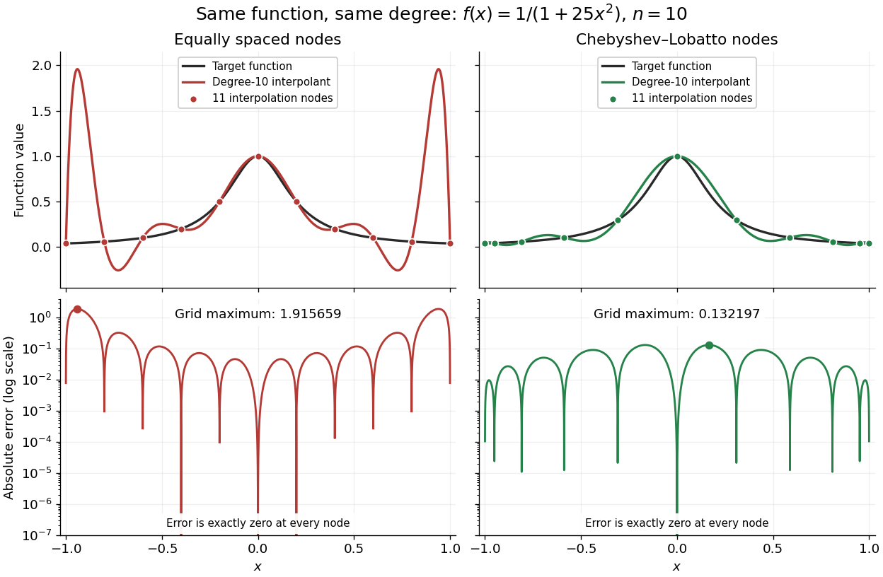
Degree-10 interpolation of the Runge function at equally spaced and Chebyshev-Lobatto nodes, with absolute errors
. Details. The polynomial interpolation error formula explains why interpolation nodes enter the analysis. If has continuous derivatives on an interval containing and all the interpolation nodes, then for a suitable in that interval,At an interpolation node the error is zero directly. Away from the interpolation nodes, both the product and the high-order derivative matter. A short proof applies Rolle's theorem repeatedly to , which vanishes at distinct points.[ref]
https://fncbook.com/polynomial/. Driscoll and Braun, Fundamentals of Numerical Computation, §9.1.2, Theorem 9.1.3
The successful comparison here does not assert that Chebyshev-Lobatto nodes solve every approximation problem for every function. The derivatives, the polynomial degree, and measurement errors still matter. The Lebesgue constant of interpolation measures worst-case amplification of nodal errors, while the polynomial reproduction error bound relates interpolation to the best uniform approximation available at that polynomial degree.
For a real continuous function on a compact interval, choose its best uniform approximation of polynomial degree at most . If its error is nonzero, the Chebyshev alternation theorem supplies ordered alternating extrema. The intermediate value theorem gives a zero of in each intervening interval. At these distinct points, the polynomial interpolant is exactly . If the best error is zero, arbitrary distinct nodes suffice. The Weierstrass approximation theorem shows that these function-dependent interpolants converge uniformly. The nodes depend on the target function; the conclusion does not provide one universal node sequence for every continuous target.
An interpolation polynomial for distinct nodes and prescribed values is a polynomial satisfying . There is a unique such polynomial of degree at most : the Lagrange interpolation polynomial constructs it explicitly, and uniqueness follows because a nonzero degree-at-most- difference cannot have distinct roots. Newton interpolation polynomials express the same object using divided differences.
A poly-infinite cyclic group has a finite subnormal series all of whose nontrivial factors are infinite cyclic groups. Intersecting its series with a subgroup again gives trivial or infinite cyclic factors; repetitions may be deleted. Splicing a kernel series with the preimage of a quotient series proves closure under extensions. Such groups are finitely presented groups: induct on the series, split the last extension by an infinite cyclic quotient, and use finite presentation of a semidirect product.
The Hirsch length of a polycyclic group counts infinite cyclic factors in a polycyclic series. Refinement shows it is independent of the series, additive in extensions, and unchanged in finite-index subgroups. A finite-index poly-infinite cyclic group has one infinite cyclic factor for each unit of Hirsch length.
Polycyclic groups are virtually poly-infinite cyclic by  Codex 0 Created 2026-10-14 Updated 2026-11-05
Every polycyclic group has a finite-index subgroup with a series whose nontrivial factors are infinite cyclic. This is the polycyclic finite-index lemma; it also supplies torsion-free finite-index subgroups. Such a subgroup is a poly-infinite cyclic group. Combining its series with the extension rule for Poincare duality groups makes it a duality group of dimension its Hirsch length.
Take every three-element subset of a four-element vertex set as a hypergraph edge. Any three-colouring repeats a colour on two vertices. A triple containing that pair cannot contain all three colours. Thus this uniform hypergraph has no polychromatic three-colouring, although each edge meets only three other edges.
Two-dimensional quantum-gravity interpretation of strings by Codex 0 Created 2026-10-14 Updated 2026-11-05
Codex 0 Created 2026-10-14 Updated 2026-11-05The Polyakov path integral integrates over string worldsheet metrics as well as embedding fields, modulo worldsheet diffeomorphisms and Weyl transformations. Summing surface topologies gives perturbative two-dimensional quantum gravity coupled to the coordinate matter fields. Gauge fixing retains worldsheet moduli and introduces ghosts; a conformal gauge is locally flat, not a global flat metric on every genus. Cancellation of the worldsheet Weyl anomaly makes the critical bosonic version consistent.
A pollen tube germination assay makes tube emergence visible outside a flower. The published Practical Biology experiment, Observing the growth of pollen tubes (Practical Biology), Technical note 3, lists florist lilies among successful materials without specifying a species. Record the actual identification; success with one sample cannot establish a universal growth rate.[ref]
Observing the growth of pollen tubes (Practical Biology). Technical note 3 and Teaching notes: material dependence and contorted versus straight tubes
Pearson's Core practical 4: Investigate the effect of sucrose concentration on pollen tube growth by Pearson Education Ltd, Teacher sheet, pp. 1–2, describes an inspectable experiment. Mix equal volumes of sucrose solution and mineral-salt medium on clean cavity slides. Dust in pollen from mature anthers with a mounted needle, record the addition time, and incubate without coverslips in covered dishes containing wet filter paper. The moist chamber reduces drying; the uncovered drops avoid oxygen limitation. Brief observations with an optical microscope at , using an eyepiece graticule calibrated against a stage micrometer, reveal tube emergence and length. Return slides to the chambers and switch off the lamp between observations to reduce heating and drying. For comparisons of sucrose concentration, use the same flower across treatments to control maturity, then repeat with other flowers.[ref]
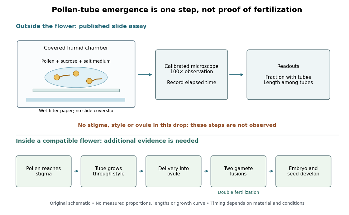
An additional proposed experimental design check is a medium-only slide: it tests whether debris is being mistaken for pollen tubes. Compare matched pollen samples at different final sucrose concentrations, keeping temperature, elapsed time and observation rules fixed. A sample known to produce pollen tubes in a previously successful medium would test whether an apparent failure comes from handling or the tested condition. These controls are questions to test, not guaranteed outcomes. A negative result cannot distinguish dead pollen from an unsuitable medium without further comparisons.
Two original calculations clarify the readout. First, take of sucrose solution and of sucrose-free medium. Assuming additive volumes, conservation of the amount of substance givesThis dilution also halves the medium's original component concentrations. Label the final molar concentration, not the starting bottle.
Second, stipulate a toy field containing pollen grains, of which have emerged pollen tubes. Its emergence fraction is . If those twelve pollen tubes have total measured length , their arithmetic mean length is . Assigning length zero to the other grains instead gives per grain. These invented numbers show why emergence fraction and mean length among emerged tubes answer different questions. Specify the denominator and the emergence criterion before counting, and avoid selecting only conspicuous long pollen tubes.
Tube emergence in a drop demonstrates growth under that medium's conditions. It observes no stigma interaction, passage through a style, delivery into an ovule, gamete fusion, or seed development. Thus a positive pollen tube germination assay does not demonstrate successful fertilization in a living flower. Its beauty is making one otherwise hidden part of sexual reproduction directly observable.[ref]
Observing the growth of pollen tubes (Practical Biology). Teaching notes: steps between pollen germination and seed formation; prepared style slides as a separate observation
For the irreducible representation of the canonical anticommutation relations determined by , a unitary one-particle map is unitarily implementable precisely when is Hilbert-Schmidt, equivalently when is Hilbert-Schmidt. The implementer is unique up to a scalar phase. The equivalent representation criterion for two polarizations is that their projections differ by a Hilbert-Schmidt operator. This yields a continuous projective unitary representation of the restricted unitary group.
For integer modes filled at indices below zero, set and on the finite-energy domain. The canonical anticommutation relations give a central term in . Summing across the filled-empty boundary gives , with . The current's level is the coefficient of this central term.
In charge , let fill all integer modes below . Its rotation energy is . The negative Heisenberg current algebra of a fermion on the circle modes create mutually commuting oscillators with . Their normalized occupation monomials applied to are orthonormal. The Jacobi triple product identifies the fermionic charge-energy generating function with , proving completeness in each finite-dimensional energy space. Thus the rotation Hamiltonian is .
A linear polarizer transmits one linear polarization and suppresses the orthogonal one. Two ideal crossed polarizers block light unless an intervening medium changes its polarization of an electromagnetic wave. A twisted nematic field effect uses this selection to convert field-driven reorientation into brightness modulation.
The Faraday effect is magnetic field-induced circular birefringence: opposite circular polarizations acquire different wave phases, rotating transmitted linear polarization. For a transparent medium with isotropy before applying the magnetic field, in the linear magnetic-response regime at fixed vacuum wavelength and temperature ,Here is the Verdet constant, is the material path length, and is the applied magnetic flux density component along the ray. This is the external bias, distinct from the oscillating magnetic field of the light itself. Michael Faraday discovered the effect in 1845.[ref]
Faraday effect. RP Photonics Encyclopedia, Faraday Effect, Rüdiger Paschotta: What is the Faraday Effect?, rotation law and discovery
Fix the sign before using the formula. On the forward path choose a right-handed Cartesian coordinate system, propagation along , and measure from toward for the electric field's oscillation line. Positive is counterclockwise in the -right, -up end view seen from , looking toward the source. Then and positive means positive rotation for positive . This convention differs from the clockwise-positive convention in optical rotation. A linear polarization line is unchanged by ; a measured orientation determines accumulated rotation only modulo , unless continuity selects a branch.
For uniform , the formula reduces to . Its appeal is that a weak change of refractive index becomes a visible change of orientation. Magnetic reversal measurement of Faraday rotation turns this into an inference of or of the magnetic field path integral. Faraday rotation on a round trip explains the directional behavior used by an optical isolator. In an astronomical cold plasma, the high-frequency limit instead leads to the rotation measure law ; that wavelength dependence is not a universal law for transparent solids.
For a finite-intensity set of mean , independent red marking with probability gives counts withDisjoint source sets give independent pairs of these counts. Refining overlapping test sets into disjoint cells then proves independence of the two whole Poisson point processes, not only their counts on one set.
Pinned article: Introduction to the OurBigBook Project
Welcome to the OurBigBook Project! Our goal is to create the perfect publishing platform for STEM subjects, and get university-level students to write the best free STEM tutorials ever.
Everyone is welcome to create an account and play with the site: ourbigbook.com/go/register. We belive that students themselves can write amazing tutorials, but teachers are welcome too. You can write about anything you want, it doesn't have to be STEM or even educational. Silly test content is very welcome and you won't be penalized in any way. Just keep it legal!
Intro to OurBigBook
. Source. We have two killer features:
- topics: topics group articles by different users with the same title, e.g. here is the topic for the "Fundamental Theorem of Calculus" ourbigbook.com/go/topic/fundamental-theorem-of-calculusArticles of different users are sorted by upvote within each article page. This feature is a bit like:
- a Wikipedia where each user can have their own version of each article
- a Q&A website like Stack Overflow, where multiple people can give their views on a given topic, and the best ones are sorted by upvote. Except you don't need to wait for someone to ask first, and any topic goes, no matter how narrow or broad
This feature makes it possible for readers to find better explanations of any topic created by other writers. And it allows writers to create an explanation in a place that readers might actually find it.
Figure 1. Screenshot of the "Derivative" topic page. View it live at: ourbigbook.com/go/topic/derivativeVideo 2. OurBigBook Web topics demo. Source. - local editing: you can store all your personal knowledge base content locally in a plaintext markup format that can be edited locally and published either:This way you can be sure that even if OurBigBook.com were to go down one day (which we have no plans to do as it is quite cheap to host!), your content will still be perfectly readable as a static site.
- to OurBigBook.com to get awesome multi-user features like topics and likes
- as HTML files to a static website, which you can host yourself for free on many external providers like GitHub Pages, and remain in full control

Figure 2. You can publish local OurBigBook lightweight markup files to either OurBigBook.com or as a static website.
Figure 3. Visual Studio Code extension installation.
Figure 5. . You can also edit articles on the Web editor without installing anything locally. Video 3. Edit locally and publish demo. Source. This shows editing OurBigBook Markup and publishing it using the Visual Studio Code extension. 
- Infinitely deep tables of contents:




All our software is open source and hosted at: github.com/ourbigbook/ourbigbook
Further documentation can be found at: docs.ourbigbook.com
Feel free to reach our to us for any help or suggestions: docs.ourbigbook.com/#contact