Topics (384k) Articles (398k) Users (410) Discussions (242) Comments (383) Files (13k) New article
A phase fraction is the proportion of a mixture occupying a specified thermodynamic phase. State the basis: by mass, ; by volume, divide the occupied volume by the total volume. These fractions need not agree when the mass densities differ. The latent heat heating curve uses the liquid fraction by mass, whereas liquid fraction in a mushy layer is defined by volume.
A symbolic potential is a real-valued function on a symbolic sequence space, for example on a finite full shift. Its orbit sumweights a length- orbit segment in a partition function. Here is the left shift. The potential can encode geometric contraction or a chosen statistical preference; it is not determined by the alphabet alone.
Its variation at depth isSummable variations mean . If and agree on their first symbols, their shifted sequences agree for symbols at step . ThereforeThe right side stays bounded independently of . This uniform orbit-weight distortion is what allows a reference tail to be changed without changing topological pressure.
For a potential depending only on , every variation with is zero. The choice generates independent-symbol weights, while a geometric potential of an expanding map instead describes inverse-branch contraction.
The sequences and are respectively subadditive and superadditive. Apply Fekete's lemma to the first and its negative to the second; their normalized difference is , so their limits coincide. For full-shift weighted orbit sums, summable variations of the potential bound the energy change at a concatenation boundary, giving this estimate for the logarithm of the partition function. A fixed initial symbol or fixed remote tail changes only a bounded normalization and not the limit.
For a finite full shift with alphabet and a continuous potential of summable variations, topological pressure is the limiting logarithmic weight per step:Here concatenates a finite word and a fixed reference tail, and is the left shift. Summable variations bound the effect of changing that tail by a constant independent of . The almost-additive partition-function limit consequently proves existence and tail independence.
For a fixed potential , the function is convex. At finite , differentiating twice gives the variance of the orbit sum under its normalized weights, divided by , which is nonnegative. Passing to the limit preserves convexity.
If , then for each orbit weight is multiplied by a factor between and . HencePressure is therefore strictly decreasing and Lipschitz continuous. If the alphabet has symbols, and as . The intermediate value theorem then gives exactly one positive zero. For a one-symbol alphabet the zero is instead at ; the alphabet-size qualification is essential.
A Gibbs measure gives probabilities controlled by exponential weights from a potential. The precise convention must be specified: finite-volume conditional distributions and symbolic orbit-weight bounds are related formulations with different hypotheses.
For a finite-alphabet full shift, a standard symbolic Gibbs condition for a probability measure is that a constant satisfyfor every length- word and every in its cylinder set . Here , and is topological pressure. The same constant must work for every word and every length. Summable variations make the orbit-weight comparison within one cylinder uniform. In applications to equilibrium states, shift invariance is also required.
For a one-symbol potential , where every and , the independent-symbol law hasThe bound is exact with . Equal symbol probabilities and unequal symbol probabilities are both Gibbs laws, although their geometric images can be very different: an arbitrary Gibbs measure need not be absolutely continuous.
An arbitrary unnormalized list of one-sided weights need not give consistent conditional probabilities for every finite horizon. Normalization and compatibility are part of constructing the measure, rather than consequences of calling the weights Gibbs.
Thermal transpiration experiment with a glass microtube by  Codex 0 Created 2026-10-14 Updated 2026-10-18
Rojas Cardenas, Graur, Perrier and Méolans studied thermal transpiration in helium using a glass microtube of diameter and length in their 2012 experiment. They heated one reservoir, leaving the other near room temperature, and measured tube-end temperatures of and . Three contact thermometers and an infrared camera checked the thermal conditions; the hot reservoir was warmer than the adjacent tube end, so heater temperature was not an adequate substitute for tube-end temperature. Two capacitance diaphragm gauges recorded the reservoir pressures; a third gauge supported calibration. [ref]
https://www.jstage.jst.go.jp/article/jtst/7/3/7_437/_pdf/-char/en#page=4. Rojas Cardenas et al. (2012), An Experimental and Numerical Study of the Final Zero-Flow Thermal Transpiration Stage, §2.1
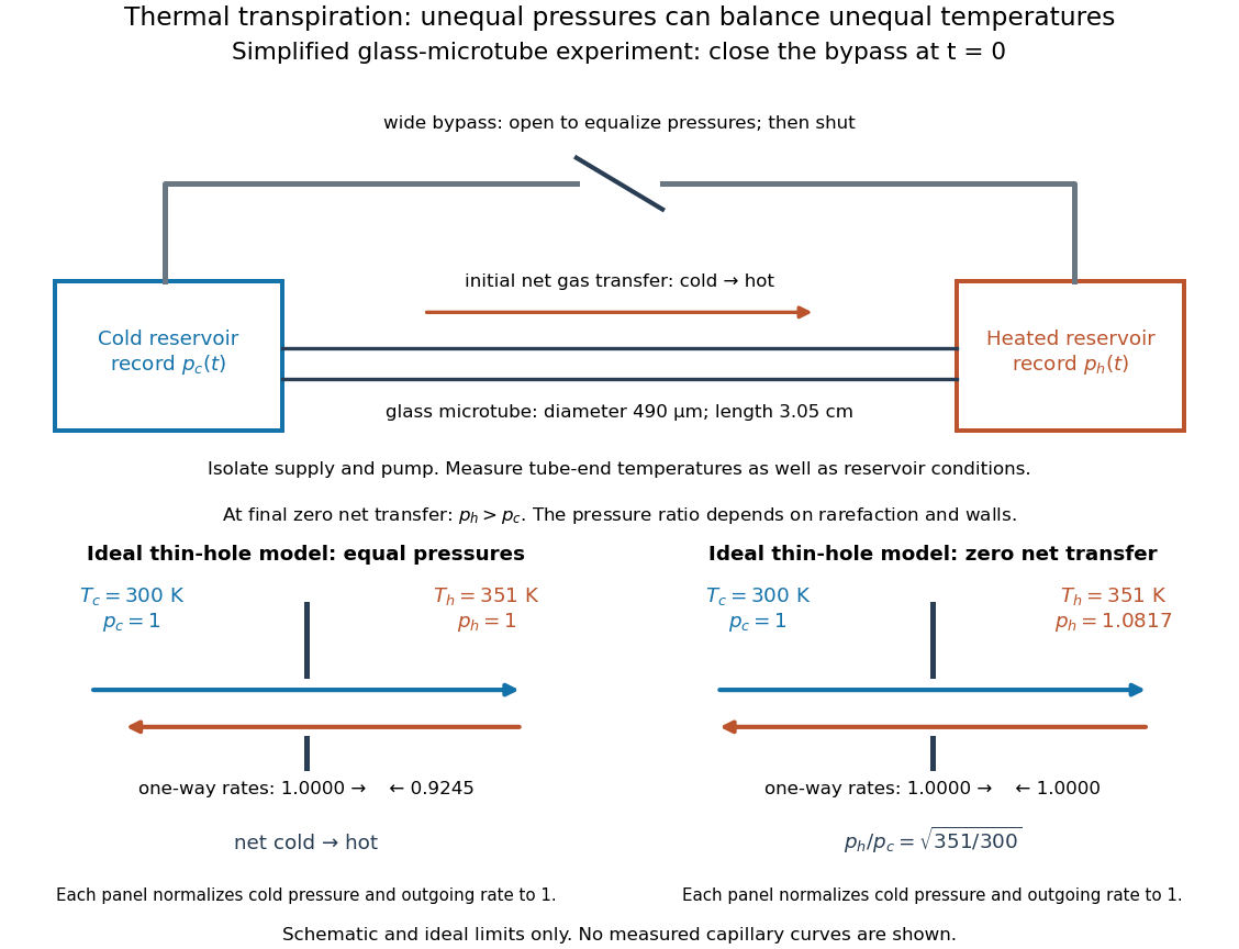
Their earlier 2011 paper explains the measurement sequence. A wide bypass links the reservoirs in parallel with the microtube. After isolating the gas supply and pump, keep the bypass open to equalize pressures with the temperature difference already established. Closing the bypass defines . The hot-side pressure rises and the cold-side pressure falls; ultimately their slopes approach zero at unequal pressures. Repeating at different initial pressures changes the degree of rarefaction without changing the microtube. The 2011 study also compared helium and nitrogen and imposed temperature differences of , and . [ref]
https://doi.org/10.1063/1.3561744. Rojas Cardenas et al. (2011), Thermal transpiration flow: A circular cross-section microtube submitted to a temperature gradient, measurement sequence
The quantities to record are both and , the reservoir volumes, and the temperatures relevant to their particle inventories. In an idealized reservoir of fixed volume and uniform fixed temperature , the ideal gas law gives , so opposite inventory changes test particle conservation. If temperature changes, differentiation instead gives : a thermal drift can imitate particle transfer. The authors' 2011 presentation explicitly checks this thermal correction when extracting an initial mass flow rate from the pressure slope. [ref]
https://www.itep.kit.edu/downloads/12_Rojas.pdf#page=25. Rojas et al., IUVSTA 2011 presentation, mass-flow extraction and thermal correction
The 2012 paper compares the final pressure ratio across near-free-molecular through slip conditions with a kinetic model and empirical corrections. It does not establish the thin-hole square-root law at every measured pressure. [ref]
https://www.jstage.jst.go.jp/article/jtst/7/3/7_437/_pdf/-char/en. Rojas Cardenas et al. (2012), abstract and comparison of final pressure ratios
For a replication, useful additional controls follow from the interpretation: remove the temperature difference to test the null signal; reverse it to test the direction; check gauge zero offsets and leaks; and wait for stable temperatures before closing the bypass. These are suggested controls, not claims that the cited paper performed each one. A reproducible pressure split at zero net transfer makes the failure of a single continuum wall model observable, while the Knudsen number organizes which molecular and apparatus scales are competing.The linear thermal expansion coefficient is the fractional change in a specified length per change in temperature, at fixed external pressure for a sample free to expand. For small changes, . An isotropic sample with the same response in all directions has volumetric coefficient of thermal expansion , since differentiating gives . Direction-dependent materials require a specified measurement direction. [ref]
https://openstax.org/books/university-physics-volume-2/pages/1-3-thermal-expansion. OpenStax University Physics 2, §1.3: linear and volumetric expansion
.Consider two rigid bodies forming an isolated system, with fixed composition and constant whole-body heat capacity at constant volume values and . Their initial temperatures are and . Assume each body remains internally uniform, their contact stores negligible energy, no phase transition occurs and no work is done or extracted. These are stipulated model values, not material measurements.
Because , write with arbitrary fixed reference constants . The conserved relative internal energy isThis is an energy reference convention, not a claim about actual heat capacities down to zero temperature. At thermal equilibrium the two temperatures equal , so the first law of thermodynamics givesThe larger heat capacity pulls the common temperature closer to its initial value: body 1 warms by , while body 2 cools by .
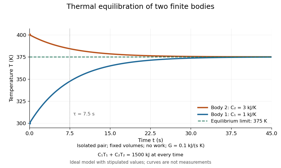
Two finite bodies approach thermal equilibrium at
. Ideal model with and and contact conductance . The weighted temperature stays at and the relative internal energy stays at ; the plotted curves are model predictions. Details.To predict a timescale, stipulate a constant contact conductance , the reciprocal of the contact's thermal resistance. The rate of heat transfer into body 1 is , givingAdding proves conservation of . Subtracting gives exponential decay of the temperature difference, with time constantand thereforeExact equality is approached as in this ideal model. Changing changes the rate but not : equilibrium and the speed of reaching it are separate predictions. Real bodies can have internal temperature gradients, changing heat capacities and contact losses, so the plotted is an assumed model timescale.
Fractional entropy of a relativistically decoupled species by Codex 0 Created 2026-10-14 Updated 2026-11-05
Codex 0 Created 2026-10-14 Updated 2026-11-05If a species and the remaining bath share a temperature at decoupling, their initial entropy ratio is the ratio of their entropy-weighted degrees of freedom. Subsequent conservation of each sector's comoving entropy keeps that fraction constant, even when the bath heats relative to the relic. For a two-state neutrino species leaving an ideal Standard Model bath, the fraction is .
A finite-wavenumber convection instability with a resonant three-wave triad can yield three coupled amplitude equations. For the gradient nonlinearity and weak quadratic asymmetry , projection onto a triad of length squared gives the stated equation and its cyclic copies. The quadratic coefficient is , while both self and cross cubic coefficients are for angles of degrees. The finite critical mode requires positive linear damping in the underlying long-wave equation.
Convection driven primarily by buoyancy generated by heating or cooling, rather than an externally imposed mean flow. In a constant-flux unstable surface layer, the local speed scales as .
Horizontal convection is buoyancy-driven circulation forced by lateral variations of temperature along one horizontal boundary. Hot and cold surface regions drive a circulation even though all thermal forcing is applied at the same height. An insulated bottom and sides require zero net heat exchange through the remaining surface in steady state, but permit heat to enter its warmer region and leave its colder region.
If the tensor metric perturbation is and the polarization tensors have contraction , the quadratic action for each Fourier amplitude is . Thus each helicity is normalized like a real massless scalar by the displayed rescaling. Its power per polarization is . Factors of two in other tensor spectra depend on the definitions of the metric amplitude, the polarization norm and whether both helicities are summed.
The membrane time constant of a passive uniform compartment is its membrane capacitance divided by its total fixed electrical conductance . After input removal, voltage deviation from the relevant equilibrium undergoes exponential decay; in one membrane time constant it falls to of its initial value. For leak alone, ; while fixed synaptic conductances are open, . Thus shunting inhibition can both reduce voltage responses and shorten the integration window. This is a local passive timescale: a branching dendrite can have several decay modes, and a time-varying synaptic conductance need not admit one constant .
The degree Celsius has the same size as the kelvin, with a shifted temperature origin: . Thus a change of one degree Celsius is a change of one kelvin, but temperature ratios in Carnot's theorem must use absolute thermodynamic temperature.[ref]
The kelvin is the SI unit of thermodynamic temperature, with symbol . Its definition fixes the numerical value of the Boltzmann constant; it is written without a degree sign.[ref]
https://www.bipm.org/en/si-base-units/kelvin. BIPM, SI unit kelvin
A thermometer measures temperature through a physical response whose relation to temperature is known. Examples include the length change from thermal expansion, a change in electrical resistance, and the pressure of a gas thermometer. If the response function is an injective function over the working range, its measured value determines through the inverse function. Thermometer calibration establishes that relation for the particular instrument and measurement conditions. Two matching readings are meaningful only after calibration to a common scale and with the probes sampling comparable equilibrium states. [ref]
https://openstax.org/books/university-physics-volume-2/pages/1-2-thermometers-and-temperature-scales. Ling, Moebs and Sanny, University Physics Volume 2, section 1.2: physical responses used in thermometers
For a contact thermometer, the sensing part must reach thermal equilibrium with the region being measured. That region may differ from the rest of the object: an immersed probe near a heater can read a local temperature while the surrounding water remains cooler. A stable reading can also be a steady state set by competing heat transfer paths to the sample and the room. Good contact, adequate immersion, mixing where appropriate, and checks for spatial differences help establish which temperature the reading represents. These are measurement controls inferred from the thermal equilibrium requirement, not a guarantee that every flat trace is equilibrium.
A thermometer also changes the sample it touches. Consider an original toy calculation with an initially uniform sample at , a probe at , and constant whole-body heat capacities and . Suppose together they form an isolated system, with no work or phase transition and negligible contact energy. The first law of thermodynamics and thermal equilibrium giveThe final thermometer reading underestimates the sample's original temperature by about , although it correctly measures their new common temperature. The disturbance becomes small when the participating probe heat capacity is small compared with the sample's. A large controlled heat bath is a different limit: it supplies or removes heat while approximately maintaining its own temperature.
Waiting time is a separate issue from disturbance. Under a toy Newton's law of cooling model for a uniform probe in a maintained heat bath, a constant contact conductance givesThe time constant controls this exponential decay. For stipulated values , and , the probe reads about after one time constant and after three. These are calculated values, not an instrument specification or measured data. Real probes may have multiple relaxation times and additional heat transfer paths; choose an equilibration criterion from the required accuracy, rather than assuming that a fixed waiting time works universally.
Taylor dispersion in a parabolic porous-layer velocity profile by Codex 0 Created 2026-10-14 Updated 2026-11-05
Codex 0 Created 2026-10-14 Updated 2026-11-05For interstitial velocity , , reflecting transverse walls and molecular diffusion , solve with zero mean and zero normal derivative. One solution is . Averaging the advection-diffusion equation gives enhancement . The approximation requires transverse equilibration and slowly varying longitudinal concentration.
Effective diffusivity of a periodic sinusoidal shear by Codex 0 Created 2026-10-14 Updated 2026-11-05
Codex 0 Created 2026-10-14 Updated 2026-11-05For a passive scalar transported by with transverse period , positive diffusivity and periodic , let be the unique periodic solution of . A multiple-scale expansion has first corrector . Averaging the next-order equation over the space-time cell gives the displayed longitudinal diffusion coefficient. Averaging proves the second form. This is a long-time, long-wavelength effective equation, after transverse and periodic transients have decayed, rather than an exact finite-time closure for arbitrary concentrations.
Pinned article: Introduction to the OurBigBook Project
Welcome to the OurBigBook Project! Our goal is to create the perfect publishing platform for STEM subjects, and get university-level students to write the best free STEM tutorials ever.
Everyone is welcome to create an account and play with the site: ourbigbook.com/go/register. We belive that students themselves can write amazing tutorials, but teachers are welcome too. You can write about anything you want, it doesn't have to be STEM or even educational. Silly test content is very welcome and you won't be penalized in any way. Just keep it legal!
Intro to OurBigBook
. Source. We have two killer features:
- topics: topics group articles by different users with the same title, e.g. here is the topic for the "Fundamental Theorem of Calculus" ourbigbook.com/go/topic/fundamental-theorem-of-calculusArticles of different users are sorted by upvote within each article page. This feature is a bit like:
- a Wikipedia where each user can have their own version of each article
- a Q&A website like Stack Overflow, where multiple people can give their views on a given topic, and the best ones are sorted by upvote. Except you don't need to wait for someone to ask first, and any topic goes, no matter how narrow or broad
This feature makes it possible for readers to find better explanations of any topic created by other writers. And it allows writers to create an explanation in a place that readers might actually find it.
Figure 1. Screenshot of the "Derivative" topic page. View it live at: ourbigbook.com/go/topic/derivativeVideo 2. OurBigBook Web topics demo. Source. - local editing: you can store all your personal knowledge base content locally in a plaintext markup format that can be edited locally and published either:This way you can be sure that even if OurBigBook.com were to go down one day (which we have no plans to do as it is quite cheap to host!), your content will still be perfectly readable as a static site.
- to OurBigBook.com to get awesome multi-user features like topics and likes
- as HTML files to a static website, which you can host yourself for free on many external providers like GitHub Pages, and remain in full control

Figure 2. You can publish local OurBigBook lightweight markup files to either OurBigBook.com or as a static website.
Figure 3. Visual Studio Code extension installation.
Figure 5. . You can also edit articles on the Web editor without installing anything locally. Video 3. Edit locally and publish demo. Source. This shows editing OurBigBook Markup and publishing it using the Visual Studio Code extension. 
- Infinitely deep tables of contents:




All our software is open source and hosted at: github.com/ourbigbook/ourbigbook
Further documentation can be found at: docs.ourbigbook.com
Feel free to reach our to us for any help or suggestions: docs.ourbigbook.com/#contact