If $\sqrt{2}=p/q$ in lowest terms, then $p^2=2q^2$ makes $p$ even. Substituting $p=2r$ then makes $q$ even, contradicting that the integers are coprime. More quantitatively, $|2q^2-p^2|\ge 1$ for every nonzero integer $q$, and factoring the difference of squares gives $|\sqrt{2}-p/q|\ge 1/(4q^2)$. To verify the constant, for $p/q\in [1,2]$ the other factor $\sqrt{2}+p/q$ is less than four; outside this interval the approximation error is at least $\sqrt{2}-1>1/4$.

In this structural use, the coordination number counts nearest neighbouring constituents. State which neighbours are counted and which ionic crystal structure is being described; it is not an ion's electric charge number.

The rock salt structure of ordinary sodium chloride has a coordination number of six for each kind of ion: six nearest neighbours of the opposite sign surround each ion along three perpendicular directions. Its conventional cubic unit cell contains four formula units; sharing corner, face, and edge sites between adjacent cells must be included in that count. Sixfold local coordination is compatible with $1:1$ overall stoichiometry.^[ref]

The checkerboard plane in the diagram is a slice through this three-dimensional arrangement. It leaves out the two nearest neighbours above and below the plane. Repeating a complete even-by-even patch gives equal numbers of signs; the displayed odd-by-odd crop has a boundary imbalance and is not a complete neutral ionic crystal or a unit cell. Other salts need not have the rock salt structure or the same coordination number.

An ATP-sensitive potassium channel couples membrane potassium conductance to cellular nucleotide state. A familiar pancreatic complex combines Kir6.2 pore subunits with SUR1 regulatory subunits. Increased intracellular ATP tends to inhibit channel opening; in a pancreatic beta cell, reduced potassium conductance can promote membrane depolarization and subsequent insulin secretion. Nucleotide regulation therefore links glucose metabolism to electrical activity, with regulatory-subunit and nucleotide-context dependence. ^[ref]

For one-dimensional inverse scattering, the Gelfand-Levitan-Marchenko equationrecovers the transformation kernel $K$ from scattering data encoded by $F$. In the convention used for the Korteweg-De Vries equation above, the potential is

Put $E_k=e^{i(kx+k^{3}t)}$, $I={\int }_L\phi (l)d\lambda (l)$ and $q=-I_x$. For the dressing operator $\mathcal{F}h=h+i{E}_k{\int }_{L}h(l)/(k+l)d\lambda (l)$, differentiating gives $\mathcal{F}(M\phi )=0$ and $\mathcal{F}(N\phi )=3ikM\phi$, where $M={\partial }_x^2-ik{\partial }_x+q$ and $N={\partial }_t+{\partial }_x^3+3q{\partial }_x$. Uniqueness of the linear integral equation therefore supplies a Lax pair. Its commutator identity is $[N,M]=-3q_{x}M+(q_t+q_{xxx}+6q{q}_x)$, which gives the KdV equation when the eigenfunction is not identically zero. Differentiation under the integral and the uniqueness assumption are essential hypotheses.

Scattering data describe connections between normalized solutions of an auxiliary spectral equation, together with any discrete spectral points and their norming data. In an inverse scattering transform, the nonlinear potential is reconstructed from these data; boundary spectral connection matrices must additionally obey a global relation.

A problem is well posed in the sense of Hadamard when a solution exists for every admissible datum, is unique, and depends continuously on the data. Failure of any condition makes it ill posed.

The X-ray transform records integrals of a function or tensor evaluation over a specified family of curves. The curve family, parametrization and any weights are part of the definition. Straight lines, geodesics and magnetic flows give different versions; their injectivity and unavoidable potential kernels depend on that geometry.

An inverse problem is an ill-posed problem if it fails any requirement of a well-posed problem: existence for every admissible datum, uniqueness, or continuity of the reconstructed object as the data change. These requirements depend on the chosen spaces and norms, not just the equation. Clason's regularization notes formulate this distinction explicitly.^[ref]

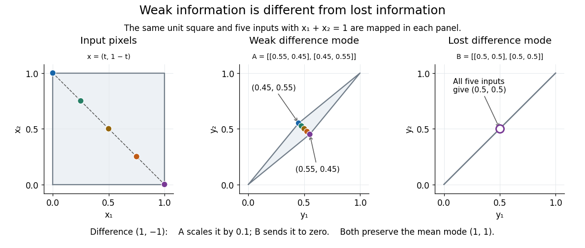
Complete averaging illustrates lost information:The difference mode $q_{-}=(1,-1{)}^T/\sqrt{2}$ belongs to the null space because $B{q}_{-}=0$. Even restricting both pixels to $[0,1]$ leaves infinitely many indistinguishable inputs. This is failure of uniqueness. Data such as $(0.51,0.49{)}^T$ also have no exact preimage under $B$, illustrating failure of existence when arbitrary two-component observations are admissible.

The two-pixel matrix $A$ in the inverse problem example has a weakly observed difference mode, not a null space mode. Its inverse is continuous: this finite-dimensional problem is a well-posed problem with noise-sensitive conditioning. Small positive singular values alone do not imply mathematical ill-posedness. In infinite-dimensional problems, positive singular values approaching zero can make inversion unbounded: unit solution modes then produce data tending to zero. This destroys continuity even without a null space. Regularization of an inverse problem must distinguish missing information from information recoverable only at the cost of amplifying measurement noise.

Tomography reconstructs an interior distribution from measurements along multiple lines or paths through it. A linear unattenuated model is the Radon transform; absorption changes it to an attenuated Radon transform.

Image deblurring reconstructs a sharper image from observations described by a blur model. In the linear model, a matrix or linear operator mixes values of the unknown image; measurement noise perturbs the observed result. The inverse problem must therefore recover attenuated distinctions while controlling amplification of measurement noise, as the two-pixel example illustrates.

For $\dot{x}=F(x,y)$ and $\dot{y}=G(x,y)$, a differentiable graph $y=h(x)$ is invariant precisely when $Dh(x)F(x,h(x))=G(x,h(x))$. This is the chain rule along a trajectory on the graph. The equation determines coefficients in a local power-series approximation of a stable manifold or unstable manifold; checking tangent directions alone does not ensure invariance.

G2 phase follows completed nuclear DNA replication and precedes mitosis. The ordinary diploid state is $2n,4C$. ^[ref]

During S phase, nuclear DNA replication produces paired sister chromatids. DNA content rises from $2C$ to $4C$, while the chromosome count remains $2n$.

During G1 phase, growth and preparation precede DNA replication. The ordinary diploid nuclear state is $2n,2C$.

The Lyman-alpha forest is the multitude of foreground Lyman-alpha absorption features in a distant quasar's spectrum, at wavelengths shorter than its own redshifted Lyman-alpha emission. The quasar supplies a bright background; intervening neutral hydrogen atoms remove photons near their local Lyman-alpha line resonance. Many dips can therefore come from one atomic transition encountered at different redshifts, rather than from many different chemical elements. Some features are instead transitions of other ions, so a dip alone does not identify Lyman-alpha absorption. This makes faint foreground gas detectable through the light it removes, even when its own emission would be difficult to see. ^[ref].

Ignoring peculiar velocity for the moment, an absorber at cosmological redshift $z_a$ puts its Lyman-alpha line atThe rest wavelength is in the ultraviolet; at $z_a=2$ it appears at $3647.01\text{A˚}$ in the optical spectrum. In a toy sightline to a quasar at $z_Q=3$, absorbers at $z_a=2,2.35,2.7$ appear at $3647.01,4072.4945,4497.979\text{A˚}$, all shortward of the quasar's Lyman-alpha emission position $4862.68\text{A˚}$. The absorbing atoms see the selected photons at their own resonance; the observed dip's redshift belongs to the foreground gas. Peculiar velocity adds a Doppler shift, so the inferred $z_a$ is not a pure distance coordinate. The rest wavelength and resonance interpretation are given in Rauch (1998), section 1.

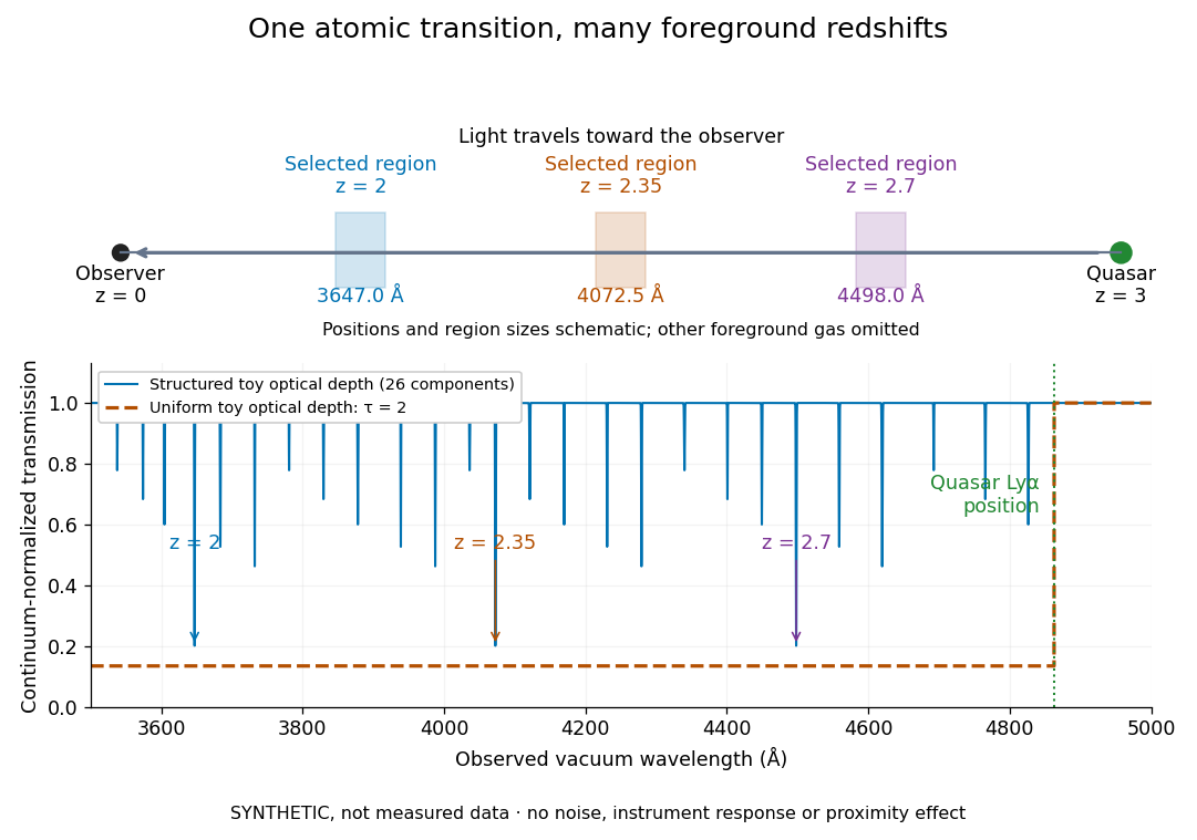
The diagram uses invented optical depths and 26 Doppler cores; three selected foreground regions are marked. Their drawn positions and sizes are schematic. The dashed comparison imposes a uniform optical depth $\tau =2$, giving transmission $e^{-2}\simeq 0.135$ throughout the chosen foreground band. It is an idealized smooth-absorption model, not a measured spectrum or a prediction of the actual intergalactic medium.

The smooth comparison explains the Gunn-Peterson effect: neutral hydrogen distributed throughout an expanding intergalactic medium can absorb continuously over a wavelength interval, because different parts of the path resonate with different observed wavelengths. The resolved Lyman-alpha forest instead has strong transmission fluctuations and distinguishable absorption lines. These need not represent isolated compact clouds: diffuse sheets and filaments in the cosmic web can generate peaks in optical depth along one line of sight. A continuously varying gas distribution can look like a collection of lines. ^[ref]. ^[ref].

An early observation makes the identification concrete. Lynds's 1971 paper analyzed six spectrograms of the quasar 4C 05.34, with emission redshift $2.877$, taken in spring 1970 using an image-tube spectrograph on Kitt Peak's 84-inch telescope. Five covered $3200$–$7500\text{A˚}$ with approximately $10\text{A˚}$ resolution; the most informative covered about $3500$–$6000\text{A˚}$ at $5\text{A˚}$ resolution. Its reproduced spectrogram shows the strong Lyman-alpha emission flanked mostly on the short-wavelength side by numerous absorption lines. Lynds tabulated their wavelengths and estimated strengths, identified five absorption redshift systems, and proposed that many remaining unidentified lines were the same Lyman-alpha line at additional redshifts. He explicitly warned about blending, an incomplete census of weak lines, and wavelength errors around $0.5$–$1\text{A˚}$. The result established a striking spectral pattern; the paper's proposed interpretation did not measure a separate physical cloud for every dip. ^[ref].

A contrasting observation demonstrates smooth, very strong absorption. Becker and collaborators (2001) used the Echelle Spectrograph and Imager on Keck II to observe the quasar SDSSp J103027.10+052455.0 at $z_Q=6.28$. Sky lines gave an instrumental full width at half maximum of about $1.8\text{A˚}$ near $8500\text{A˚}$, or spectral resolving power $R\simeq 4700$. After sky subtraction and flux calibration, the mean continuum-normalized transmission over $8450$–$8710\text{A˚}$ was $0.0038\pm 0.0026$, consistent with zero; this corresponds to absorption redshifts approximately $5.95$–$6.16$. They identified a Gunn-Peterson trough. Crucially, resonant Lyman-alpha absorption is so sensitive that even a small neutral fraction can make transmission undetectable: the trough alone does not establish a mostly neutral intergalactic medium or uniquely date reionization. ^[ref].

What a spectrum constrains is a radiative transfer problem. For an ideal foreground screen with negligible emission into the observed beam, the intrinsic continuum-normalized transmission isHere $F$ is spectral radiative flux, $F_{\mathrm{cont}}$ is its unabsorbed continuum, $\tau$ is optical depth, $n_{\mathrm{HI}}$ is neutral hydrogen number density, and $N_{\mathrm{HI}}$ is neutral hydrogen column density along proper path length $\ell$. A Voigt profile model constrains redshift, column density and a velocity width together. A nearly black line has lost much of its sensitivity to further increases in optical depth; blending and an uncertain continuum can also admit different fitted components. Finite spectral resolving power and noise limit which widths and weak features can be measured. ^[ref]. ^[ref].

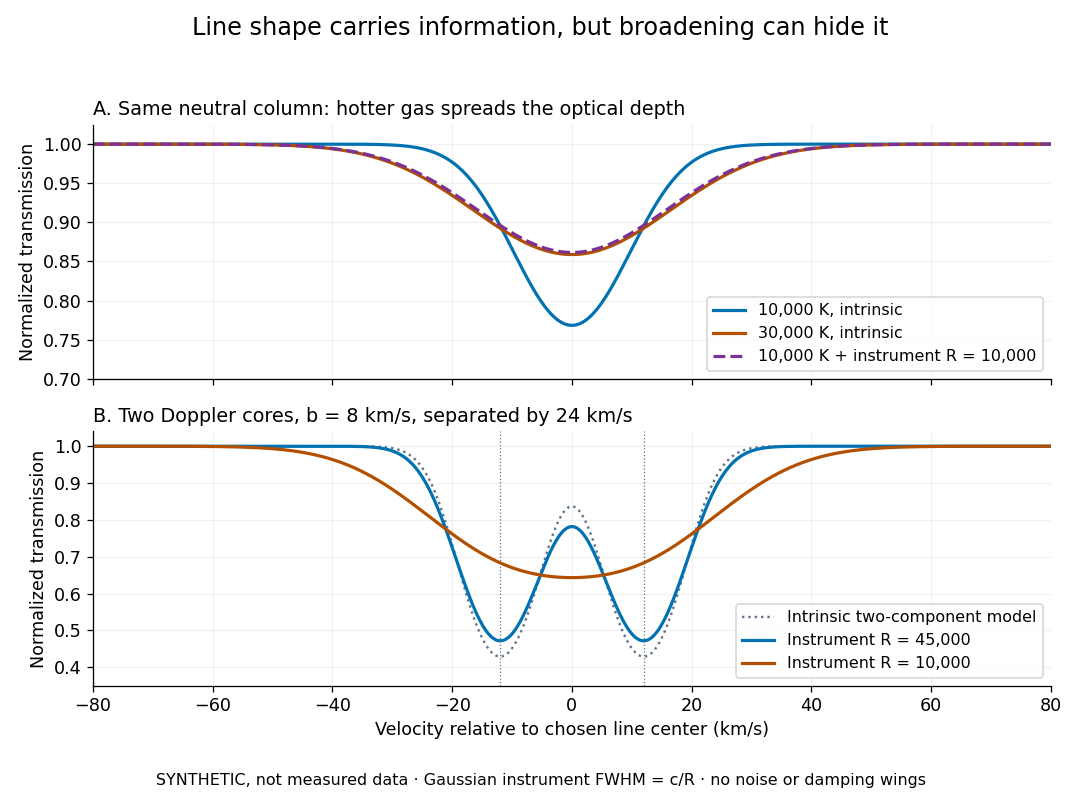
For a purely thermal Doppler core, use the velocity convention $\tau (v)\propto \exp [-(v-v_0{)}^2/b^2]$. The Maxwell-Boltzmann velocity distribution then giveswhere $k_B$ is the Boltzmann constant, $T$ is temperature and $m_{\mathrm{H}}$ is a hydrogen atom's mass. This $b$ is $\sqrt{2}$ times the Gaussian distribution's standard deviation. Higher temperature spreads the same column density over more velocities. An instrument also broadens a line: locally, for a nearly flat continuum, the recorded transmission is approximately the convolution of $\mathcal{T}$ with the normalized instrumental response, not the exponential of a convolved optical depth. A Gaussian response with full width at half maximum $c/R$ has standard deviation $c/[R\sqrt{8\log 2}]$, where $c$ is the speed of light and $R$ the spectral resolving power.

The upper model fixes the integral $\int \tau (v)dv$, hence the neutral hydrogen column density for this transition, while changing temperature. A cooler line blurred by an instrument resembles a warmer intrinsic line. The lower model has two equal Doppler cores separated by $24\mathrm{km}{\mathrm{s}}^{-1}$: reducing spectral resolving power merges them into one apparent feature. Both panels use invented profiles, Gaussian instrumental responses, and no noise or damping wings. They illustrate an inverse problem, rather than measurements of temperature or a universal relation between a dip and a cloud.

Better observations provide the inputs to that inverse problem. Kim, Cristiani and D'Odorico (2001) analyzed three quasars with the VLT's UVES spectrograph. For HE2217–2818, Table 1 records $z_Q=2.413$ and $16200\mathrm{s}$ of exposure in the $3050$–$3860\text{A˚}$ setup in October 1999. Isolated thorium-argon lamp lines measured $R\simeq 45000$; the data were resampled into $0.05\text{A˚}$ bins, with signal-to-noise ratios about $45$–$50$ per pixel over $3550$–$4050\text{A˚}$. They fitted a local polynomial continuum, fitted Voigt profiles, and compared statistics of the transmitted flux. Their analysis excluded the region near the quasar to avoid the quasar proximity effect and used the interval between its Lyman-beta and Lyman-alpha emission to reduce confusion with other Lyman-series absorption. Features below $N_{\mathrm{HI}}=10^{12.5}\mathrm{c}{\mathrm{m}}^{-2}$ became confused with noise, setting their adopted lower column density limit. Figure 1 shows the measured spectrum, fitted profiles and residuals. This was a calibrated absorption measurement, with explicit selection limits. ^[ref].

Even after instrumental correction, a width need not be purely thermal Doppler broadening. Hubble flow across extended gas, peculiar velocity structure and unresolved blends can contribute. If an isolated line's intrinsic width obeys $b^2=b_{\mathrm{th}}^2+b_{\mathrm{nt}}^2$ with an independent Gaussian nonthermal contribution $b_{\mathrm{nt}}^2\ge 0$, then $T\le m_{\mathrm{H}}{b}^2/(2k_B)$; $b=25\mathrm{km}{\mathrm{s}}^{-1}$ gives a computed upper bound about $3.79\times 10^4\mathrm{K}$. A complex blend need not satisfy this single-component model. Noise can also bias the fitted widths of weak lines. This is why the thermal cutoff of Lyman-alpha line widths, calibrated against gas models, is more informative than assigning a temperature to every dip. ^[ref].

Finally, neutral hydrogen column density is not total gas mass density. In a pure hydrogen approximation, with gas optically thin to ionizing radiation and nearly fully ionized in photoionization equilibrium, the Lyman-alpha forest photoionization scaling giveswhere $n_{\mathrm{H}}$ counts all hydrogen nuclei, $\Gamma$ is the photoionization rate, $\alpha (T)$ is the radiative recombination coefficient and $x_{\mathrm{HI}}=n_{\mathrm{HI}}/n_{\mathrm{H}}$ is the neutral fraction. At fixed temperature and $\Gamma$, doubling $n_{\mathrm{H}}$ quadruples $n_{\mathrm{HI}}$; doubling $\Gamma$ halves it. These computed examples explain both the sensitivity to density contrast and the ambiguity: stronger absorption can mean denser gas, weaker ionizing radiation, a different temperature, or more path length. The Jeans-length ionization correction for the Lyman-alpha forest adds a size model rather than an independently measured depth. Optically thick Lyman limit systems and damped Lyman-alpha systems require different treatment. ^[ref]. ^[ref].

The beauty of the Lyman-alpha forest is that a spectrum converts otherwise faint foreground gas into a sequence of markers through cosmic time. With a model of radiative transfer, velocities, ionizing radiation and the temperature-density relation of photoionized intergalactic gas, its transmission statistics probe the cosmic web and gas thermal history. A single line of sight remains one narrow sample, not a unique three-dimensional density map. ^[ref].

The cosmic ionizing background is the diffuse radiation field capable of photoionization of intergalactic gas. Its specific intensity depends on source luminosity functions, ionizing photon escape fractions, cosmological redshifting, and radiative transfer through absorbers. Quasars and star formation supply major contributions with different spectral shapes and evolution.

Diffuse gas in photoionization equilibrium is often approximately described by the displayed temperature-density contrast relation. Photoheating and expansion cooling produce its thermal history. It is an empirical model for low-density gas, not the adiabatic equation of state of every intergalactic phase. Lyman-alpha forest line widths constrain both the temperature at a reference density and the slope through their lower envelope.

The Weierstrass transform is Gaussian convolution, $Wf(x)=(4\pi {)}^{-1/2}{\int }_{\mathbb{R}}{e}^{-(x-y{)}^2/4}f(y)dy$. It smooths appropriate functions and is the heat semigroup at unit time. The Brownian transition semigroup uses variance-$t$ Gaussian kernels and therefore supplies the scaled time family.