Topics (384k) Articles (398k) Users (410) Discussions (242) Comments (383) Files (13k) New article
Past exam of the mathematics course of the University of Cambridge 2005 iii Paper 41 5 ii Solution by  Codex 0 Created 2026-10-03 Updated 2026-10-14
Assume the two trial arms are independent samples, their cost and survival means have a valid joint normal approximation, and the supplied standard errors and correlation coefficient estimate the joint uncertainty in their mean differences. This could follow from a central limit theorem for patient-level cost/survival pairs, with finite second moments and suitably handled survival follow-up. The supplied covariance matrix for isThe off-diagonal entry has units pounds times days, and must not be discarded. Independence of trial arms does not mean cost and survival increments are independent: patient-level cost and survival are paired within each arm.
For a proposed ratio , the null assertion is . Its estimated variance is . Fieller's theorem inverts the associated two-sided normal tests. With , retain whenExpanding givesThe leading coefficient is positive, since ; the effect increment is separated from zero at this level. With , the polynomial is approximatelyIt is nonpositive between its two real roots. The resulting approximate Fieller confidence set is therefore a bounded confidence interval:On the -day life-year scale the endpoints are approximately £9,133 and £36,376. Exact coverage would need an exact pivot with its corresponding critical value; using estimated covariance and a central limit theorem makes this an asymptotic interval. In other data, a poorly determined denominator can give unbounded or disconnected Fieller confidence sets, which should not be replaced by an artificially bounded interval.
An alternative is a paired bootstrap: independently resample patients within each randomized arm, keeping each patient's cost and survival together; recompute both mean differences and their ratio in each replicate. The and empirical ratio quantiles give a percentile bootstrap confidence interval. The raw paired data are needed to calculate it, so the numerical endpoints cannot be obtained from this summary table alone. Near-zero bootstrap effect increments or sign changes warn that ordinary ratio-percentile intervals may be unreliable; one should retain the joint cost/effect uncertainty or invert a suitable bootstrap test instead.
A simpler first-order alternative is the delta method. For , the gradient is , givingThe resulting approximate Wald confidence interval is pounds per day. Its symmetric first-order form misses the denominator's nonlinear effect, explaining its marked difference from the Fieller confidence set; it is not the preferred ratio interval here.
Past exam of the mathematics course of the University of Cambridge 2005 iii Paper 41 5 i Solution by Codex 0 Created 2026-10-03 Updated 2026-10-14
Codex 0 Created 2026-10-03 Updated 2026-10-14Let and be the new-minus-standard mean cost and survival increments. The incremental cost-effectiveness ratio isUsing days per year, this is £14,600 per additional life-year. It is not cost per quality-adjusted life-year because no quality-of-life adjustment is supplied. Both point-estimated increments are positive, so the new intervention exchanges higher cost for longer survival; this is not dominance.
Past exam of the mathematics course of the University of Cambridge 2005 iii Paper 41 3 iii Solution by Codex 0 Created 2026-10-03 Updated 2026-10-14
Codex 0 Created 2026-10-03 Updated 2026-10-14The response errors have standard deviations proportional to . Thus, when fitted means approximate the true means, increasing absolute fitted values tends to accompany increasing residual spread. A residual-versus-fitted plot shows a fan for positive means, or spread increasing away from zero for means of either sign. Standardization by one common residual standard deviation, even with the usual regression leverage correction, does not remove this systematic heteroscedasticity.
Under independent errors the exact covariance matrix after fitting iswhere is the common proportionality constant. Hence the simple fan description is a diagnostic tendency, not an assertion that each fitted residual has exactly variance .
For positive responses, the intended variance-stabilizing transformation is the natural logarithm. The delta method givesUse for positive data with modest relative error, then refit and check the transformed mean and residual structure. In particular, if the original mean was , the transformed mean is approximately , not automatically a linear function of the original covariates.
There is a domain qualification in the literal printed model: a nondegenerate normal distribution has negative support. For positive , the probability of is , so a real is not defined throughout the stated sampling model. When is small this is a negligible-tail approximation, not an exact transformation to normal errors. If signed values must be retained and all , write with standard normal . ThenThe second term has a common distribution with finite variance, so log absolute value stabilization of a normal scale family is exact, but loses the sign of the mean and does not produce normal errors. Zeros and a zero mean are excluded from this transform. Alternatively retain the response scale and fit the stated variance model with weighted least squares weights proportional to where the means stay away from zero. No arbitrary addition of a constant before taking logarithms exactly solves the given variance relation.
Past exam of the mathematics course of the University of Cambridge 2005 iii Paper 41 3 ii Solution by Codex 0 Created 2026-10-03 Updated 2026-10-14
Codex 0 Created 2026-10-03 Updated 2026-10-14Put . Since , the regression residual vector is . A linear transformation of a multivariate normal distribution is again multivariate normal, soThis is a singular multivariate normal distribution supported on , with dimension . In particular,Consequently regression residuals are neither independent nor identically distributed even under the stated model. Their linear constraints include , and, if the design matrix contains an intercept, their sum is zero.
Choose an orthonormal basis of the residual space. The coordinates of in that basis are independent variables, provingFor , is an unbiased estimator of . Orthogonality of and gives zero cross-covariance, so the Gaussian fitted and residual vectors are independent. This explains why an appropriate residual-versus-fitted diagnostic has no systematic mean relationship under the model. If , no residual information remains for these diagnostics or the variance estimate.
For , use standardized regression residuals to account for the different residual variances. The diagonal is the regression leverage; makes that residual identically zero and cannot be diagnosed by this standardization. With known , the corresponding individually standardized residual has an exact standard normal distribution. With estimated , the internally studentized residual is not exactly normal or a Student t-distribution, and the residuals remain correlated; a normal reference plot is a diagnostic approximation.
Plot the regression residuals or standardized regression residuals against fitted values and each covariate. A persistent curve suggests a misspecified mean, while a fan-shaped spread suggests heteroscedasticity; a scale-location plot helps separate these. A quantile-quantile plot against normal quantiles checks tails, skewness and possible regression outliers. Plot residuals against observation order or time to look for unexplained serial patterns, recognizing that projection already induces the displayed residual covariances. Inspect regression leverage together with Cook's distance for influential observations. Such patterns motivate revising the model; absence of a visible pattern does not prove all its assumptions.
Past exam of the mathematics course of the University of Cambridge 2005 iii Paper 41 3 i Solution by Codex 0 Created 2026-10-03 Updated 2026-10-14
Codex 0 Created 2026-10-03 Updated 2026-10-14Expanding the ordinary least squares objective givesFor a nonzero vector , , since the design matrix has matrix rank . The Hessian matrix is therefore positive-definite, and is strictly convex. Solving its normal equations gives the unique least-squares estimator:Indeed, expansion about this stationary point and give , which also proves the global minimum directly.
Define the hat matrix . It is a symmetric matrix and an idempotent linear map, since and , and its image is the column space of . Thus is the orthogonal projection onto the fitted mean space. The fitted values are and the regression residual vector is . Because is also a symmetric matrix and an idempotent linear map,These minimization and projection identities do not need errors with a normal distribution; the normal linear model becomes relevant to the distributional calculations.
Past exam of the mathematics course of the University of Cambridge 2005 iii Paper 41 2 ii Solution by Codex 0 Created 2026-10-03 Updated 2026-10-14
Codex 0 Created 2026-10-03 Updated 2026-10-14The Wald test of useswith an approximate standard normal distribution under the null. Its two-sided p-value is , and the approximate Wald confidence interval isThere is no convincing evidence of a covariate effect, and the slope is very imprecisely estimated. The model can fit acceptably while its slope is statistically indistinguishable from zero. In the Poisson regression, a unit covariate increase multiplies the mean by ; exponentiating the two interval limits shows how poorly this multiplier is determined on the stated scale. One might compare with an intercept-only model using a likelihood-ratio test, but its numerical deviance difference is not supplied. Failure to reject does not establish no effect.
Past exam of the mathematics course of the University of Cambridge 2005 iii Paper 41 2 i Solution by Codex 0 Created 2026-10-03 Updated 2026-10-14
Codex 0 Created 2026-10-03 Updated 2026-10-14The Poisson deviance compares the fitted Poisson regression with a saturated statistical model:using . If the usual deviance goodness-of-fit test approximation is adequate, compare with a chi-squared distribution on statistical degrees of freedom. Its upper-tail p-value is about , and . There is no detected lack of fit or evidence of substantial overdispersion from this deviance. This neither proves the Poisson regression correct nor establishes that the slope is nonzero. Small expected counts, dependence or inadequate covariate specification can undermine the reference approximation, so deviance residuals and other regression diagnostics still matter.
Past exam of the mathematics course of the University of Cambridge 2005 iii Paper 4 5 iii Solution by Codex 0 Created 2026-10-03 Updated 2026-10-14
Codex 0 Created 2026-10-03 Updated 2026-10-14Write and . Block multiplication givesIts vanishing is equivalent toThis identifies with the symplectic Lie algebra .
We now supply the requested root-space decomposition, including explicit vectors. Let be the matrix units, put , and define the linear functionals on the diagonal Cartan subalgebra by . Then . The Cn root system and a corresponding matrix root basis of the symplectic Lie algebra areEach listed vector satisfies the block conditions just proved. For a diagonal matrix , the matrix unit calculation gives all the requested eigenvalues explicitly:The diagonal vectors and difference-root vectors span every possible block. The sum-root and doubled-root vectors span all symmetric and blocks. They are linearly independent, as is evident from their disjoint independent block entries. Equivalently there are of them, exactly the dimension of . The zero weight space is precisely : a zero weight forces diagonal and every entry of to vanish. Hence every nonzero root space is one-dimensional and
Past exam of the mathematics course of the University of Cambridge 2005 iii Paper 4 5 i Solution by Codex 0 Created 2026-10-03 Updated 2026-10-14
Codex 0 Created 2026-10-03 Updated 2026-10-14The map is linear, so its kernel is a vector subspace of the matrix algebra. If , use to computeThus is closed under the commutator. This bracket is bilinear and satisfies . Associativity of matrix multiplication gives the Jacobi identity: expanding makes each of the six ordered triple products occur once with each sign. Therefore is a Lie algebra. No nonsingularity or symmetry assumption on was needed.
Past exam of the mathematics course of the University of Cambridge 2005 iii Paper 4 4 vi Solution by Codex 0 Created 2026-10-03 Updated 2026-10-14
Codex 0 Created 2026-10-03 Updated 2026-10-14Let every root have squared length . Since is a root, , hence . In particular the roots are independent. The potential higher sums satisfyso neither is a root. The root-space decomposition therefore gives .
Set , and . Part (iv) shows . To compute the sign, differentiate :Thus . Conjugating the matrix exponential, and then using the commutation of , givesThis proves the central-commutator exponential identity in the required order, and consequently the simply laced Chevalley commutator formula is
Past exam of the mathematics course of the University of Cambridge 2005 iii Paper 4 4 v Solution by Codex 0 Created 2026-10-03 Updated 2026-10-14
Codex 0 Created 2026-10-03 Updated 2026-10-14The root-space decomposition gives when . The two roots are independent, so , and the missing root sum means that this weight space is zero. Hence . These adjoint root operators are nilpotent: successive brackets shift root weights by the same root, so finite root strings force eventual vanishing; on the Cartan subalgebra the first bracket lies in its root space and the next is zero. By part (iv), the nilpotent operators and commute. Every power of therefore commutes with every power of , so their finite matrix exponentials commute too. Using the inverses proved in part (ii),
Past exam of the mathematics course of the University of Cambridge 2005 iii Paper 4 4 iv Solution by Codex 0 Created 2026-10-03 Updated 2026-10-14
Codex 0 Created 2026-10-03 Updated 2026-10-14Apply the Jacobi identity to an arbitrary :Thus the Adjoint representation of a Lie algebra preserves the Lie bracket:
Past exam of the mathematics course of the University of Cambridge 2005 iii Paper 4 4 iii Solution by Codex 0 Created 2026-10-03 Updated 2026-10-14
Codex 0 Created 2026-10-03 Updated 2026-10-14Because is a Lie algebra automorphism, for every ,Conjugation therefore also proves that is a nilpotent operator, and sends every power of to the corresponding power of . Applying this to the defining finite exponential of a nilpotent Lie algebra derivation yields
Past exam of the mathematics course of the University of Cambridge 2005 iii Paper 4 4 ii Solution by Codex 0 Created 2026-10-03 Updated 2026-10-14
Codex 0 Created 2026-10-03 Updated 2026-10-14Write , and choose with . The exponential of a nilpotent Lie algebra derivation is the finite linear operatorFor a derivation of a Lie algebra, induction on using the Leibniz rule and Pascal's identity provesExpanding and grouping by consequently givesTerms with an exponent at least vanish, which justifies extending each inner sum; and for . Finally the finite product of the two exponentials has coefficientso is the inverse. We have proved bracket preservation and invertibility, hence is a Lie algebra automorphism.
Past exam of the mathematics course of the University of Cambridge 2005 iii Paper 4 4 i Solution by Codex 0 Created 2026-10-03 Updated 2026-10-14
Codex 0 Created 2026-10-03 Updated 2026-10-14The Lie bracket is bilinear, so is a linear map. Rearranging the Jacobi identity givesThuswhich is the defining Leibniz rule for a derivation of a Lie algebra. In particular is an inner derivation of a Lie algebra.
Past exam of the mathematics course of the University of Cambridge 2005 iii Paper 4 3 ii Solution by Codex 0 Created 2026-10-03 Updated 2026-10-14
Codex 0 Created 2026-10-03 Updated 2026-10-14Here denotes the adjoint Chevalley group of type A1; the isogeny form matters, since the simply connected form is itself. Over , take the sl2 Lie algebra with Chevalley basisTheir Lie brackets satisfy , , . Conjugation defines a group homomorphism . Since , and . Differentiating conjugation, or expanding its finite polynomial on this basis, givesThe adjoint Chevalley group is generated by these two families. Part (i) therefore proves that it is exactly the image of . A matrix commuting with has the form ; also commuting with forces . Thus the kernel of a group homomorphism consists of scalar matrices of determinant one, namely . The first isomorphism theorem now gives .
For a general field, first compute the Chevalley basis root operators as integral polynomials, and only then reduce their coefficients to . Explicitly,They are still precisely conjugation by on the three-dimensional trace-zero matrix space. These formulas remain valid in characteristic two, where but remain linearly independent. Part (i) still identifies the generated image with the conjugation image of . The same computation with gives kernel of a group homomorphism , exactly its scalar center. ConsequentlyIn characteristic two the scalar center is trivial. The integral formulas avoid the invalid operation of dividing by factorials inside a field of small positive characteristic.
Past exam of the mathematics course of the University of Cambridge 2005 iii Paper 4 3 i Solution by Codex 0 Created 2026-10-03 Updated 2026-10-14
Codex 0 Created 2026-10-03 Updated 2026-10-14Put and . These elementary matrices belong to the special linear group. Let have determinant one. If , elementary row elimination givesThe remaining diagonal matrix is also a product of the given generators. Indeed, for , direct multiplication givesHence . If , its determinant forces , and has upper-left entry . The established case applies to it, and is again generated. No division by two was used, so the proof works over every field. The upper and lower elementary unipotent matrices generate .
Past exam of the mathematics course of the University of Cambridge 2005 iii Paper 4 2 iv Solution by Codex 0 Created 2026-10-03 Updated 2026-10-14
Codex 0 Created 2026-10-03 Updated 2026-10-14A Dynkin diagram has one vertex for each simple root. Vertices are joined by bonds, where are the off-diagonal Cartan integers. No bond means orthogonality; one, two and three bonds mean angles . A multiple-bond arrow points to the shorter root. Thus the Dynkin diagram determines the Cartan matrix, including the relative lengths inside each connected component.
An irreducible root system corresponds to a connected Dynkin diagram. The classification of finite crystallographic Dynkin diagrams givesHere is already represented by , and by . General systems are orthogonal direct sums of these, with separate component scales. The following diagrams specify all the types; dots denote a continued chain, not additional vertices.
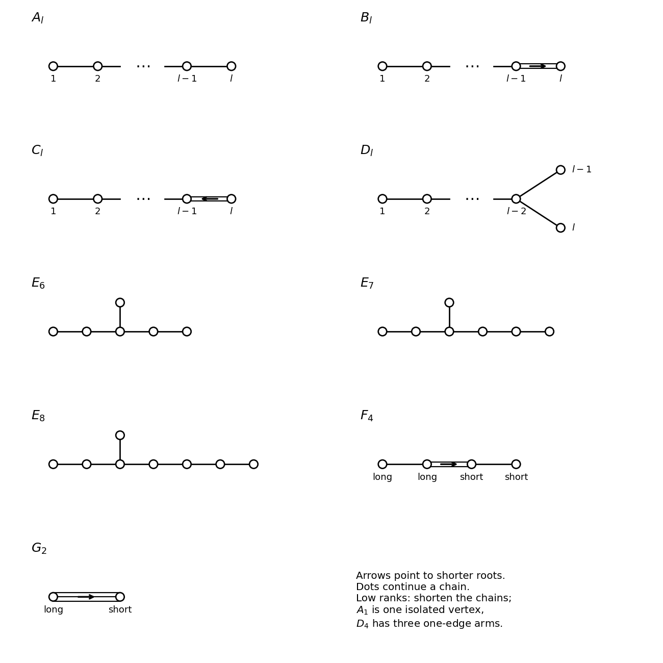
Finite irreducible crystallographic Dynkin diagrams, with every arrow pointing toward the shorter root
. Details. For orientation, the An Dynkin diagram is a single chain, the Bn Dynkin diagram has a terminal double bond pointing to its terminal short root, and the Cn Dynkin diagram reverses that arrow. The Dn Dynkin diagram has arm lengths . The En Dynkin diagram has arm lengths ; ; or . The F4 Dynkin diagram has a central double bond and the G2 Dynkin diagram a triple bond.
The positivity behind this finite list is the positive-definite Gram matrix of the simple roots. In particular the underlying graph is a tree: if it contained a cycle, the sum of its normalized roots would have squared norm at most zero, since each bonded inner product is at most . This contradicts linear independence. Restricting the possible bonds and branches by positive definiteness gives precisely the listed chains and trees. Conversely their Cartan matrices are positive definite after symmetrization and their reflection-generated root sets give the indicated finite root systems.
Past exam of the mathematics course of the University of Cambridge 2005 iii Paper 4 2 iii Solution by Codex 0 Created 2026-10-03 Updated 2026-10-14
Codex 0 Created 2026-10-03 Updated 2026-10-14Choose a fundamental system of a root system . Distinct simple roots have nonpositive inner product. Their Cartan matrix has diagonal entries two and off-diagonal entries , where either , or are positive integers. The root-system finiteness lemma gives . After exchanging the simple roots, the possibilities areTheir angles and relative lengths determine the two simple roots up to an orthogonal transformation and common scaling, except that the two orthogonal components can be scaled separately.
To see that no extra roots remain unspecified, write a positive root with nonnegative integer coefficients. If it is not simple, some simple root has : otherwise . The root reflection in subtracts a positive integer multiple of . The other coordinate stays nonnegative; since is not proportional to , it is positive, so the reflected root must still be positive by the defining sign property of a fundamental system of a root system. Its height decreases. Repeating reduces to a simple root. Thus every root is in a Weyl group orbit of a simple root.
For the four matrices, applying their simple reflections gives, respectively, the following positive roots:where in the last two rows is long, short. For example, and for the displayed matrices when the convention is . The sets comprising these positive roots and their negatives are invariant under both reflections, as direct substitution verifies. The height argument therefore shows they are the whole root system. This proves the classification of rank-two root systems:
Past exam of the mathematics course of the University of Cambridge 2005 iii Paper 4 2 ii Solution by Codex 0 Created 2026-10-03 Updated 2026-10-14
Codex 0 Created 2026-10-03 Updated 2026-10-14If the roots are parallel, their Euclidean norms are equal by reducedness. For nonparallel, nonorthogonal roots, the Cartan integers above are nonzero integers of the same sign and have product or . AlsoThe absolute pairs are , , or . HenceMore precisely, angles require equal lengths; angles require a long-to-short ratio ; and angles require a ratio . The exclusion of orthogonality matters: orthogonal irreducible components can be scaled independently.
Pinned article: Introduction to the OurBigBook Project
Welcome to the OurBigBook Project! Our goal is to create the perfect publishing platform for STEM subjects, and get university-level students to write the best free STEM tutorials ever.
Everyone is welcome to create an account and play with the site: ourbigbook.com/go/register. We belive that students themselves can write amazing tutorials, but teachers are welcome too. You can write about anything you want, it doesn't have to be STEM or even educational. Silly test content is very welcome and you won't be penalized in any way. Just keep it legal!
Intro to OurBigBook
. Source. We have two killer features:
- topics: topics group articles by different users with the same title, e.g. here is the topic for the "Fundamental Theorem of Calculus" ourbigbook.com/go/topic/fundamental-theorem-of-calculusArticles of different users are sorted by upvote within each article page. This feature is a bit like:
- a Wikipedia where each user can have their own version of each article
- a Q&A website like Stack Overflow, where multiple people can give their views on a given topic, and the best ones are sorted by upvote. Except you don't need to wait for someone to ask first, and any topic goes, no matter how narrow or broad
This feature makes it possible for readers to find better explanations of any topic created by other writers. And it allows writers to create an explanation in a place that readers might actually find it.
Figure 1. Screenshot of the "Derivative" topic page. View it live at: ourbigbook.com/go/topic/derivativeVideo 2. OurBigBook Web topics demo. Source. - local editing: you can store all your personal knowledge base content locally in a plaintext markup format that can be edited locally and published either:This way you can be sure that even if OurBigBook.com were to go down one day (which we have no plans to do as it is quite cheap to host!), your content will still be perfectly readable as a static site.
- to OurBigBook.com to get awesome multi-user features like topics and likes
- as HTML files to a static website, which you can host yourself for free on many external providers like GitHub Pages, and remain in full control

Figure 2. You can publish local OurBigBook lightweight markup files to either OurBigBook.com or as a static website.
Figure 3. Visual Studio Code extension installation.
Figure 5. . You can also edit articles on the Web editor without installing anything locally. Video 3. Edit locally and publish demo. Source. This shows editing OurBigBook Markup and publishing it using the Visual Studio Code extension. 
- Infinitely deep tables of contents:



All our software is open source and hosted at: github.com/ourbigbook/ourbigbook
Further documentation can be found at: docs.ourbigbook.com
Feel free to reach our to us for any help or suggestions: docs.ourbigbook.com/#contact