Topics (384k) Articles (398k) Users (410) Discussions (242) Comments (383) Files (13k) New article

A complex network is a graph model of an interacting system whose connectivity has nontrivial structure relevant to its behavior. The phrase does not specify one mathematical graph class: degree heterogeneity, clustered neighborhoods, community organization or changing connectivity may be important depending on the application.
For example, two graphs can have the same numbers of vertices and edges but very different shortest-path graph distances. A six-cycle has average degree two and diameter three; two disjoint triangles also have average degree two but lack paths between the two components. Their equal mean degree conceals a decisive connectivity difference.
Network science therefore uses several measurements and compares them with explicit random graph models. Labels such as small-world network or scale-free network express additional quantitative hypotheses; they should be tested rather than inferred merely because a diagram looks complicated.
A calculated net value is the difference between a measured weighing value, gross or net, and a preset tare value. The key distinction is the origin of the subtracted quantity: it is entered or recalled numerically rather than necessarily being a freshly measured tare for that individual container. OIML R76-1:2006 defines these terms separately from an ordinary net indication after operation of a tare device.[ref]
Write the arithmetic aswhere is the stored preset tare value. Here the weighing values are expressed as mass estimates, for example in kilograms; they are not forces expressed in newtons. The instrument determines mass using gravity under its measurement model.[ref]
For a chosen packaging example, let a loaded container give and let the stored nominal container tare be . The calculated net value is then . If this particular empty container actually has mass , its contents have ideal net mass . The calculated indication overestimates that value by . The subtraction has been performed correctly; the discrepancy arises because a nominal tare was substituted for an individual one.
More generally, let the true contents' mass be , the actual container mass be , and the measured gross value be , where is measurement error. ThenRepeating weighings can assess variation in , but it does not by itself remove an incorrectly chosen . A useful check therefore weighs representative empty containers as well as repeating loaded measurements. Report the stored tare and what it represents along with the result. This makes the physical assumptions behind a calculated net value visible rather than treating a precise-looking display as evidence that every container has the nominal tare mass.
The fixing operation in a nested Markov model turns a random vertex of a conditional acyclic directed mixed graph into a fixed input and transforms its probability kernel. A vertex is fixable if no other vertex in its bidirected-connected district of an acyclic directed mixed graph is a descendant of . Graphically, fixing removes edges with an arrowhead at and moves from the random to the fixed vertex set.[ref]
For a positive Markov kernel , the transformation divides by the conditional factor for given its district's other vertices and the parents of that district. Fixed arguments are retained as kernel inputs. Fixability is what permits the resulting object to be a normalized kernel over the remaining random variables. Valid fixing sequences must check this condition again after each step.
Temporal averaging in nail clippings is the mixing of material formed or transported at different times into one measured sample. A clipping has finite length, width and thickness. Even perfect chemical measurement of the whole sample need not resolve the timing of a short exposure.
A primary nail-growth experiment followed file marks near the proximal fold in 22 young adults over one to three months.[ref]
Growth rate of human fingernails and toenails in healthy American young adults by S. Yaemsiri and others. Abstract, Methods
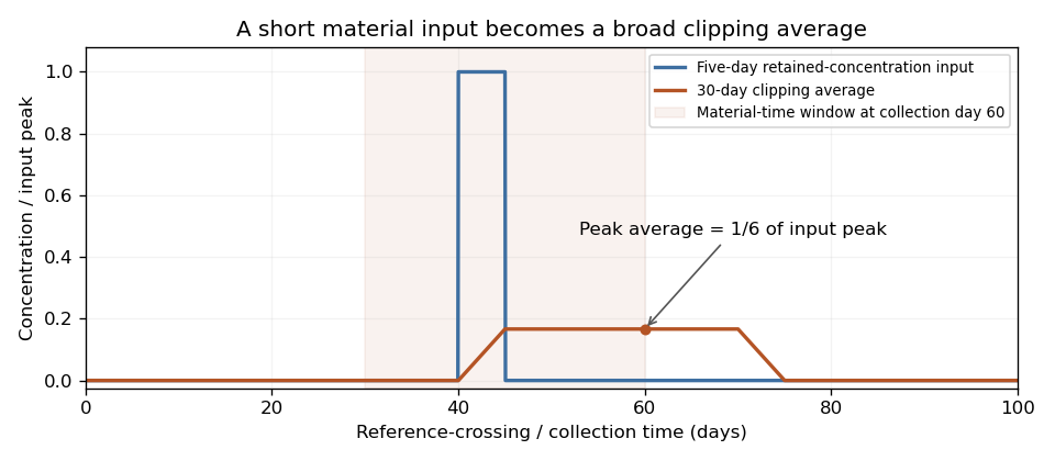
Such displacement measurements constrain the transport clock. Relating a chemical concentration to an earlier exposure requires additional assumptions about incorporation, retention and contamination.For an original ideal advection model, let material cross a reference at time with concentration , thereafter retained unchanged. At constant speed , a segment between positions and at collection time contains reference-crossing times from to . If mass per unit length is uniform, its measured concentration isThis is a shifted moving average, equivalently a convolution with a rectangular window. Its clock is reference crossing; formation in the hidden nail matrix may precede that crossing.
For a 3 mm segment at stipulated speed 0.10 mm/day, days. If a hypothetical incorporated concentration equals for only five days and zero otherwise, the largest possible clipping average is . A broad, low measured peak can therefore result from a short, high input without any chemical decay. These values illustrate the model rather than an observed exposure record.
Spatial weighting of nail-clipping exposure records becomes important when thickness, width or density varies: the average is weighted by material mass, not distance alone. Variable growth further distorts the time window. A wider segment generally mixes a longer history, while repeated analyses of the same segment improve analytical precision without shortening that history.
Record clipping extent, material orientation, collection date and how growth was measured. Comparing several separately retained segments can provide more time information than pooling them, but recovering a unique exposure history remains an inverse problem unless the transport and retention model is sufficiently constrained.
A NACA four-digit airfoil encodes three quantities: maximum airfoil camber in hundredths of the airfoil chord, its position in tenths of the airfoil chord, and nominal maximum airfoil thickness-to-chord ratio in hundredths. Thus NACA 2412 means , and ; NACA 0012 has zero airfoil camber and the same nominal thickness ratio.[ref]
With , the airfoil mean camber line isFor a symmetric airfoil, take directly; do not divide by the zero position parameter. The half-thickness follows the polynomial in trailing edge. If , the upper/lower coordinates areThickness is placed along a normal vector to the mean line, rather than simply added vertically.[ref]
For an original NACA 2412 calculation at , the mean-line slope is zero, and the standard finite-edge polynomial gives . Hence the surface points are approximately and in chord-normalized coordinates. A 12-percent designation does not mean the section is 12 percent thick at every chordwise position.
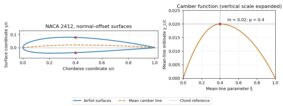
NACA 2412 mean camber line and surfaces constructed by normal offsets. Original evaluation of the stated four-digit equations.
Details. The trailing-edge convention must also be specified. The usual coefficient leaves a small finite thickness; the modified closes the endpoint. With a sloping mean line, the upper and lower endpoint coordinates can differ in both components, so directional measurement of trailing-edge thickness must state which separation it reports. These constructions define geometry, not a universal aerodynamic performance curve.
An intrafusal muscle fibre is a specialized skeletal muscle fibre within a muscle spindle. Its mechanical state is monitored by endings of sensory neurons, contributing to proprioception, and motor input adjusts that state. The ordinary force-producing extrafusal muscle fibres lie outside the muscle spindle. Intrafusal contraction therefore helps regulate a sensory apparatus as well as changing local tension.
In a cat soleus preparation, researchers repetitively stimulated a single motor fibre supplying a muscle spindle, then imposed a ramp stretch while recording a primary sensory ending. Prior motor stimulation produced an extra burst of impulses at the start of the stretch. A subsequent stretch abolished this after-effect, whereas without that stretch it could persist for more than a minute.[ref]
Two stretches with the same imposed movement can thus produce different sensory signals because the intrafusal muscle fibres have different recent activation histories. The authors proposed persistent interactions between actin and myosin as a mechanism; that proposal should be distinguished from the directly recorded impulses.[ref]
After-effects of fusimotor stimulation on the response of muscle spindle primary afferent endings by M. C. Brown and others. Abstract, observation 5, proposed intrafusal filament mechanism
Cardiac muscle is the specialized striated muscle of the heart. Its contractile cells are mechanically connected and electrically coupled at intercalated discs. Mechanical connections transmit force, while gap junctions help electrical excitation spread between cells.[ref]
Excitation and contraction are related but distinct stages. Changes in membrane potential regulate calcium handling, and calcium enables the actin-myosin machinery to generate force. A sinoatrial node normally sets the pace for the coordinated sequence, rather than an independent motor neuron commanding each beat.
This separation explains why an electrical recording and a measurement of pumping answer different questions. An electrocardiogram reports summed electrical activity; contraction also depends on cellular mechanics, filling and the loads against which the heart pumps.
The external anal sphincter is the ring of skeletal muscle surrounding the distal anal canal. Its contraction helps maintain faecal continence; its motor neurons allow voluntary squeezing as well as reflex control. It works alongside the smooth muscle of the internal anal sphincter, so continence depends on coordinated structures rather than one isolated ring.[ref]
Anatomy and Physiology 2e by J. Gordon Betts and others. Section 23.5, The Large Intestine, Anal Canal
Branches of the pudendal nerve supply the external anal sphincter. Dissection of 28 cadavers found a local nerve plexus near the sphincters in five, illustrating why a schematic nerve route need not capture every individual's branching. Preserving muscle alone therefore does not guarantee preservation of its motor supply.[ref]
Anatomy of the pudendal nerve and its terminal branches: a cadaver study by Steven E. Schraffordt and others. Abstract, Results: inferior rectal and perineal interconnections
The piriformis muscle is a deep skeletal muscle connecting the anterior sacrum to the upper femur. It passes through the greater sciatic foramen and helps rotate the extended thigh outward and abduct the flexed thigh. Its position makes it a useful landmark: the sciatic nerve usually emerges below it, although the relationship varies between people.[ref]
An anatomical variant alone does not establish a cause of pain. Adam L. Bartret and colleagues classified sciatic nerve routes on 783 hip magnetic resonance imaging examinations; variants occurred in about 19%, without a statistically significant association with a recorded diagnosis of piriformis syndrome. This observation separates a visible anatomical difference from evidence that the difference explains symptoms.[ref]
Cycle-gain uncertainty describes uncertainty in the product of the multipliers achieved over repeated chemical multiplication reaction cycles. Its size depends on cycle-gain correlation: environmental or reagent effects shared across cycles behave differently from independent cycle variation.
For positive multipliers , write and . Then , soFor small relative errors, is approximately the standard deviation of . This applies the correlated-input uncertainty propagation framework to the product model.[ref]
An original intermediate-correlation model sets . Grouping equal separations givesFor , and , the bracket is8.25, giving relative standard uncertainty approximately0.0574. Independent cycles would give0.040, while completely shared log-error would give0.080. Specifying only the uncertainty of each individual cycle leaves total-gain uncertainty undetermined.
If the log-multipliers are jointly normally distributed, has a log-normal distribution. With ,These exact relations under the stipulated distribution distinguish the mean gain from its median when variation is substantial.
Estimate correlations from a justified shared-input model or appropriately replicated sequences. Common calibration, reagent variation and cycle-dependent depletion may contribute. Adding more ideal cycles can increase nominal gain while making the final measurement uncertainty more sensitive to those shared inputs.
The dissolved formazan recovery fraction is the fraction of a specified amount of formed formazan that is represented as dissolved product in the solution being measured. Definefor a model in which the same chemical product is conserved apart from incomplete dissolution or loss. The denominator and the stage at which it is established must be stated. Product formation, product recovery and the optical response per dissolved amount are distinct parts of an MTT assay.
The manufacturer's procedure forms product crystals before solubilization and multiwell optical measurement.[ref] A lower signal can therefore arise even when the same amount of product was initially formed.
For a homogeneous solution obeying the Beer-Lambert law in a fixed optical path,If complete recovery would give net absorbance , a matched observation of gives under that model. This inference requires the reference amount, molar absorption coefficient, volume and path length to be valid for the sample. A different solvent response or erroneous background can otherwise mimic incomplete recovery.
Formazan recovery identifiability is the central limitation: the optical observation alone determines the product , not its two factors. For example, arbitrary amount units formed with and units formed with give the same dissolved amount. Repeating the same optical measurement more precisely does not separate these explanations.
A known-product addition can test the recovery of that addition at a chosen processing stage. For matched optical conditions, the expected increment is , and the observed-to-expected increment estimates the recovery of the added product. An addition after dissolution does not test losses that occurred before it. Nor does a plateau after further mixing prove complete recovery without an independent amount reference.
An MTT formazan solubilization check should consequently record where product was added or formed, which liquid was retained, dilution, solvent and optical geometry. Microplate fill-height optical cancellation can change the volume dependence of the readout, but it does not restore product that was discarded or establish cell viability.
Pinned article: Introduction to the OurBigBook Project
Welcome to the OurBigBook Project! Our goal is to create the perfect publishing platform for STEM subjects, and get university-level students to write the best free STEM tutorials ever.
Everyone is welcome to create an account and play with the site: ourbigbook.com/go/register. We belive that students themselves can write amazing tutorials, but teachers are welcome too. You can write about anything you want, it doesn't have to be STEM or even educational. Silly test content is very welcome and you won't be penalized in any way. Just keep it legal!
Intro to OurBigBook
. Source. We have two killer features:
- topics: topics group articles by different users with the same title, e.g. here is the topic for the "Fundamental Theorem of Calculus" ourbigbook.com/go/topic/fundamental-theorem-of-calculusArticles of different users are sorted by upvote within each article page. This feature is a bit like:
- a Wikipedia where each user can have their own version of each article
- a Q&A website like Stack Overflow, where multiple people can give their views on a given topic, and the best ones are sorted by upvote. Except you don't need to wait for someone to ask first, and any topic goes, no matter how narrow or broad
This feature makes it possible for readers to find better explanations of any topic created by other writers. And it allows writers to create an explanation in a place that readers might actually find it.
Figure 1. Screenshot of the "Derivative" topic page. View it live at: ourbigbook.com/go/topic/derivativeVideo 2. OurBigBook Web topics demo. Source. - local editing: you can store all your personal knowledge base content locally in a plaintext markup format that can be edited locally and published either:This way you can be sure that even if OurBigBook.com were to go down one day (which we have no plans to do as it is quite cheap to host!), your content will still be perfectly readable as a static site.
- to OurBigBook.com to get awesome multi-user features like topics and likes
- as HTML files to a static website, which you can host yourself for free on many external providers like GitHub Pages, and remain in full control

Figure 2. You can publish local OurBigBook lightweight markup files to either OurBigBook.com or as a static website.
Figure 3. Visual Studio Code extension installation.
Figure 5. . You can also edit articles on the Web editor without installing anything locally. Video 3. Edit locally and publish demo. Source. This shows editing OurBigBook Markup and publishing it using the Visual Studio Code extension. 
- Infinitely deep tables of contents:




All our software is open source and hosted at: github.com/ourbigbook/ourbigbook
Further documentation can be found at: docs.ourbigbook.com
Feel free to reach our to us for any help or suggestions: docs.ourbigbook.com/#contact