An order-parameter space is the set of allowed equilibrium values of an order parameter after accounting for the relevant symmetry breaking. When a symmetry group $G$ leaves a selected state invariant only under a subgroup $H$, the distinct symmetry-related states are often represented by the quotient $G/H$.

For a planar magnet with a fixed nonzero magnetization magnitude and free direction, the space is a circle. For a nematic orientation, opposite directions represent the same state, giving a different space. Its topology constrains possible topological defects; the physical identification of states matters as much as the number of coordinates.

An energy-normalized pulse profile separates an optical pulse's temporal shape from its total laser pulse energy. For nonnegative radiant power $P(t)$ and finite $U=\int P(t)dt>0$, define $p(t)=P(t)/U$. Then $p$ has units inverse time and integrates to one. The radiant energy in a time interval is $U$ times the integral of $p$ over that interval.^[ref]

For an original two-lobe example, let $p=1/(8\mathrm{ns})$ during $0<t<2\mathrm{ns}$ and $p=3/(8\mathrm{ns})$ during $5<t<7\mathrm{ns}$, with zero values elsewhere. The two integrals are $1/4$ and $3/4$. Choosing $U=4\mathrm{nJ}$ gives powers $0.5$ and $1.5\mathrm{W}$, and energies $1$ and $3\mathrm{nJ}$. Multiplying $U$ by two doubles both powers without changing $p$.

The temporal energy centroid of an optical pulse is $\int tp(t)dt$ when this moment exists. Here it is $(1/4)(1)+(3/4)(6)=4.75\mathrm{ns}$, in the gap between lobes. An energy centroid need not be a location of maximum power.

Mathematically, $p$ is a probability density function, but its weighting here is energy over time. It is not automatically a measured photon-arrival distribution, particularly when photon energies vary. A zero-energy trace cannot be normalized this way, and a noisy baseline-corrected trace with negative excursions is not automatically a nonnegative density. The Gaussian pulse energy and peak power article gives one normalized shape family.

An optical pulse pedestal is lower-level optical power extending around a pulse's dominant short peak. It can precede the peak, follow it or extend on both sides. A broad pedestal can carry substantial laser pulse energy while barely changing the peak's full width at half maximum. Optical pulse temporal contrast describes the relative power levels; integrated energy also depends on how long each contribution persists.

For an original power-profile model, choose a central rectangular contribution of height $P_0$ and duration $\tau$, together with a pedestal of height $\alpha P_0$ and duration $T>\tau$, centred at the same time. Let $0<\alpha <1$. The peak power is $(1+\alpha )P_0$, while the pedestal lies below half of that value. The power FWHM is therefore still $\tau$, butThese are stipulated additive power contributions, not a rule for adding coherent electric fields.

Set $\alpha =10^{-3}$ and $T=1000\tau$. The pedestal then contains half the total energy even though its power is about a thousand times below the main peak. With $P_0=1\mathrm{MW}$ and $\tau =1\mathrm{ps}$, each contribution carries $1\mu \mathrm{J}$. The peak-to-pedestal power ratio is exactly $(1+\alpha )/\alpha =1001$ in this example. An inverse convention would quote a small pedestal-to-peak ratio instead; state which contrast definition is being used.

A measurement needs temporal range as well as dynamic range. A narrow scan can miss broad wings, while a readout that resolves only the peak can bury a pedestal in its own background. A commercial example is the Sequoia third-order cross-correlation instrument, whose manufacturer identifies temporal-contrast measurement as its purpose and separately specifies scan range and temporal resolution.^[ref] The cited instrument description establishes the measurement approach; the numerical profile above is an independent model.

A real optical pedestal must also be distinguished from detector baseline subtraction errors. Blocked-beam and reference measurements characterize the detector background, while a suitable optical measurement tests whether low-level light accompanies the pulse. A detection time gate that excludes a pedestal changes the admitted energy relative to a detector integrating the full waveform.

An optical prepulse is a secondary optical pulse arriving before the reference main pulse. The sign of its delay is part of the definition: choose the main pulse at $t=0$, so a prepulse has negative arrival time. A weak earlier pulse and an equally weak optical postpulse can affect a target differently when the material retains a response to the earlier illumination. Temporal order therefore carries information that one total laser pulse energy does not.

An original separated rectangular-profile example uses a main pulse of duration $100\mathrm{fs}$ and a prepulse of duration $10\mathrm{ps}$ centred $50\mathrm{ps}$ earlier. Let the prepulse's peak radiant power be $10^{-4}$ of the main peak. The optical pulse temporal contrast is $10^4$, but the energy ratio isThus the prepulse carries $1/101\approx 0.990\%$ of the two-pulse energy. If the main pulse carries $1\mathrm{mJ}$, the prepulse carries $10\mu \mathrm{J}$. These stipulated disjoint power profiles have no field-overlap term, and the main pulse's full width at half maximum does not reveal the earlier contribution.

A temporal diagnostic needs both sufficient delay coverage and calibrated dynamic range. The single-shot third-order correlator paper motivates its asymmetric response by contrasting it with the symmetric second-order trace, which loses the distinction between before and after.^[ref] Its delay axis still needs a known physical reference. A third-order pulse correlation ghost from a real postpulse can appear on the prepulse side; interpreting every small lobe as earlier light would be incorrect.

Repeating the measurement while varying an independently characterized optical delay helps assign temporal order. Record the detector baseline subtraction, coverage and response width along with the trace. A nondetection means a limit within those measurement conditions, rather than proof of zero early optical energy.

An optical postpulse is a secondary optical pulse arriving after the chosen main pulse. Specify the delay, relative peak radiant power, duration and collected laser pulse energy: a relative peak alone does not determine the energy of a differently shaped replica. It is distinct from an extended optical pulse pedestal and from electronic ringing from a photodetector.

A transparent plate provides a concrete mechanism. At normal incidence, a transmitted replica that makes one additional internal round trip has approximate delaywhere $\ell$ is plate thickness and $n_g$ is its group refractive index. Neglect absorption, dispersion and overlap, and let each internal reflection retain power fraction $R$. The first delayed replica then has approximately $R^2$ times the directly transmitted energy. This etalon round-trip delay can create a physical optical echo.

For an original chosen $\ell =1.2\mathrm{mm}$, $n_g=1.5$ and $R=0.04$, the delay is about $12\mathrm{ps}$ and the energy ratio is $0.0016$. A $2.0\mathrm{mJ}$ main pulse would be followed by a $3.2\mu \mathrm{J}$ replica under that model. The historical single-shot correlator experiment deliberately inserted a BK7 etalon to generate and detect such a delayed pulse.^[ref]

Changing the plate thickness tests the delay prediction; changing optical alignment tests whether a stray reflection is involved. A third-order intensity autocorrelation can distinguish temporal sides under its model, while a symmetric second-order intensity autocorrelation cannot alone assign a feature to a prepulse or postpulse. An opposite-delay correlation feature may instead be a third-order pulse correlation ghost; it need not identify another physical pulse.

A Raman microscope combines an optical microscope with Raman spectroscopy to measure a spectrum from a localized specimen region. A microscope objective focuses a laser and collects scattered light; rejection filters suppress the intense excitation line, and a spectrometer separates the remaining wavelengths for detection. A facility instrument at the National University of Singapore supports both single-point measurements and Raman mapping.^[ref]

In a common backscattering arrangement, the same objective supplies excitation and collection. Moving the specimen or focus associates each Raman spectrum with a position, so a chosen spectral band can map chemical or structural variation. Confocal microscopy can additionally reject some out-of-focus light; a small map step by itself does not establish correspondingly fine spatial resolution.

For an original wavelength calculation, illuminate at ${\lambda }_0=532\mathrm{nm}$ and observe a Stokes Raman shift of $1000\mathrm{c}{\mathrm{m}}^{-1}$. The scattered wavelength satisfiesBoth reciprocal wavelengths must use the same length unit. The spectrometer measures the shifted light, while a filter suppresses the much brighter Rayleigh scattering near $532\mathrm{nm}$. Spectral resolution determines how nearby spectral features separate; objective focusing and the detection geometry determine spatial discrimination.

A concrete coupled apparatus placed a hydrated mouse bone in a mechanical tester mounted on a Raman microprobe stage. It followed mineral-band changes during elastic loading, connecting local molecular response with specimen mechanics.^[ref] Interpreting such a measurement requires the specimen position, loading conditions and laser exposure to be controlled. Local heating, fluorescence and instrumental response can change a recorded spectrum; focused illumination is not automatically non-destructive.

A stereomicroscope is an optical microscope that sends distinct views of the same specimen to the two eyes through separate viewing channels. The views originate at slightly different directions, producing stereo disparity that supports stereoscopy. Two microscope eyepieces alone do not establish stereo imaging: splitting one image into identical copies supplies no second viewpoint.

A two-objective arrangement uses separate microscope objective assemblies whose viewing directions converge on the specimen. A shared-objective arrangement can instead preserve two distinct viewing bundles through one main objective. The distinction concerns how the two perspectives are formed, rather than the number of eyepieces. A primary manufacturer manual gives a concrete two-path example: its S-series optics have a10° convergence angle and a compact lower assembly providing access around the specimen.^[ref]

For an original geometric illustration, take two viewing rays inclined by $\pm \alpha$ to the normal of a reference plane. A feature at height $h$ above that plane has ray intersections displaced in opposite directions by $h\tan \alpha$, so their separation isWith total convergence angle $2\alpha =10^{\circ }$ and $h=1\mathrm{mm}$, the separation is about0.175mm. This back-projected reference-plane geometry illustrates stereoscopic triangulation; it is not a specification of human depth accuracy or a universal pixel-to-height calibration. Actual image coordinates also depend on each channel's optics and alignment.

The distinct viewpoints are useful when positioning a fine tool near a surface, inspecting a small mechanical assembly or distinguishing raised features from flat markings. Illumination reflected from an opaque surface makes many such specimens accessible without preparing a thin transmitting section. The microscope working distance determines how much physical room remains between the instrument and the focused specimen, which matters when a probe or tool must enter that space.

For measurement, retain the magnification setting and calibrate the relevant channel with a stage micrometer. A scale calibration in a reference plane does not automatically convert stereo displacement into height; that requires the viewing geometry or a separate height calibration. Increasing magnification also does not guarantee improved diffraction-limited resolution. The purpose of the second view is geometric information, alongside the instrument's ability to resolve and magnify structure.

The microscope working distance is the clearance between the front of a microscope objective and the specified nearest specimen or cover surface when the specimen is in focus. The exact reference surfaces belong with the manufacturer's specification. For a coverslip-corrected objective, the primary manufacturer definition measures free working distance to the coverslip surface facing the front lens, with the focus at the opposite side.^[ref]

Working distance is a physical access constraint. It determines whether a tool can reach the focused specimen and whether a raised holder edge interferes with the objective. It differs from focal length, which is an optical property referenced to the relevant principal plane, and from microscope parfocal distance, which relates the objective mounting reference to the focused specimen plane. Their reference points are not interchangeable.

For an original geometric model in air, put the front principal plane at axial coordinate0, the front lens surface at−3mm and the focused specimen surface at−12mm. The object distance from the principal plane is12mm, but the lens-to-specimen working clearance is9mm. If a mounting shoulder is at+30mm, its distance to the specimen is42mm. These stipulated dimensions illustrate three different lengths; they are not specifications for a commercial objective.

For another example, suppose an objective has2.0mm free clearance to a coverslip, and a holder rim projects1.2mm above that same reference surface into the objective's lateral sweep. The simple axial clearance over the rim is0.8mm before accounting for its shape, tilt and positioning errors. Knowing only the magnification would not supply this clearance calculation. A fixture's geometry must be checked against the actual objective envelope.

Microscope depth of field instead describes a range of specimen depths judged sufficiently in focus under a stated imaging criterion. A generous working distance does not establish that a thick object is all sharply resolved at once. Conversely, a specimen can be in focus with very little physical clearance.

Optical conditions still matter: cover thickness, immersion medium and refractive index must match the objective design if its intended image performance is to be achieved. A numerical aperture or magnification value alone does not determine every clearance and optical-correction requirement. The manufacturer's objective-labeling document discusses these specifications separately.^[ref]

The microscope depth of field is the range of specimen depths judged acceptably sharp for a fixed imaging configuration and focus setting. It is an object-space tolerance defined by a sharpness criterion. It differs from microscope working distance, a physical clearance, and from image-space depth of focus. The accepted range depends on numerical aperture, wavelength, detector/display sampling and the criterion used to judge blur.

An original geometric model makes the criterion explicit. Let a local light cone have object-side half-angle $\alpha$. An axial defocus $\Delta z$ gives blur diameter approximately $b_{\mathrm{blur}}=2|\Delta z|\tan \alpha$. If acceptable object-space blur diameter is at most $b$, the symmetric depth range isThis cone model ignores diffraction and aberrations; it provides a stated geometric estimate, not a universal microscope specification.

For $b=2\mu \mathrm{m}$, refractive index $n=1$ and numerical aperture $n\sin \alpha =0.25$, the total range is about7.75µm. Raising the aperture to0.50 with the same blur criterion reduces it to about3.46µm. The manufacturer's iris discussion describes this tradeoff qualitatively: closing the aperture increases depth of field while reducing resolving power.^[ref]

In a diffraction-limited comparison, choosing a tolerable blur scale proportional to $\lambda /\mathrm{NA}$ and using $\tan \alpha \approx \mathrm{NA}/n$ at small angle yields a depth scale proportional to $n\lambda /{\mathrm{NA}}^2$. The prefactor depends on the stated sharpness criterion. It should not be treated as one exact range independent of contrast, sampling or the way the image is assessed.

For a simple acceptance example, suppose the adopted total range is6µm and a nominally flat inspected surface varies from−4 to+4µm about a center focus. The8µm extent does not fit inside that6µm interval. Moving focus shifts which parts qualify but does not increase the interval width. A larger-looking image also does not prove better diffraction-limited resolution or a larger axial acceptance range.

Record whether a quoted depth is total or one-sided, and keep the optical configuration and blur/contrast criterion with it. Otherwise two reported values can differ because they describe different acceptance tests rather than different objective performance.

The microscope parfocal distance is the specified axial distance from an objective's mechanical mounting reference to the focused specimen plane in its intended optical arrangement. Matching this distance helps objectives on a common mount place their focused object planes near the same location. It is a mechanical/optical interface dimension, rather than the microscope working distance between the front end and its specified near surface.

A primary manufacturer example shows two objectives with the same45mm parfocal distance and mounting-thread specification but visibly different body diameters and access geometries. The shared distance therefore does not imply identical front-end clearance.^[ref]

For an original coordinate example, put the mounting reference at $z=0$ and the focused specimen plane at $z=-45\mathrm{mm}$. An objective front surface at−35mm leaves10mm clearance to an uncovered flat specimen; a different objective front surface at−44.4mm leaves0.6mm. Both have45mm mounting-reference-to-focus separation in this stipulated arrangement. Comparing only their parfocal distances would conceal the clearance difference.

Nominal agreement also does not establish perfect focus after every exchange. If actual focused-plane separations are45.00 and45.03mm, keeping the specimen and mounting plane fixed leaves30µm of focus mismatch. Under a stipulated total acceptable microscope depth of field of5µm centered at focus, that mismatch exceeds the axial tolerance. A fine focus adjustment or a characterized offset is then needed to compare sharply focused images.

The focal length is another length with another reference: the relevant principal plane, rather than the mounting shoulder. Magnification, tube-lens arrangement, cover correction and immersion conditions also need to match the instrument design. A shared thread or parfocal distance alone does not establish all those optical compatibilities.

For metrology, identify the mounting reference, focused specimen plane and intended optical configuration before comparing distances. A focus test on a flat reference at the same stage setting can characterize interchange offsets. The resulting axial-offset information is distinct from an image-scale calibration made with a stage micrometer.

Separating power imbalance from mode mismatch in optical beating requires more information than a single modulation-depth reading. In the optical heterodyne modulation depth model, two effects multiply:The power ratio controls one term, while $\gamma$ describes the mode-overlap factor in optical heterodyne detection. A low beat depth can result from either effect or both.

Measure each arm separately with the same detector and collection geometry, subtracting dark current. For sufficiently close optical frequencies with the same detector responsivity, let the separate currents be $I_s$ and $I_{\mathrm{LO}}$. After correcting the receiver's beat-frequency response,This consistency bound for separately measured heterodyne arm powers requires $I_{\mathrm{beat},\mathrm{pk}}\le 2\sqrt{I_s{I}_{\mathrm{LO}}}$. An apparent value above unity indicates inconsistent calibration, background treatment, conditions or model assumptions.

For an original example, separate currents are $0.40$ and $0.10\mathrm{mA}$. Their power-imbalance limit is $m_{\max }=0.80$. A corrected beat depth $m=0.56$ means peak beat current $0.28\mathrm{mA}$ and overlap $|\gamma |=0.70$. If the electrical chain instead attenuates the beat amplitude by $0.75$ relative to DC and that effect is ignored, the apparent depth becomes $0.42$ and inferred overlap $0.525$.

NIST's physical receiver experiment matched the two optical modes and received photocurrent contributions; it separately corrected electrical loss and impedance mismatch when inferring receiver response and modulation.^[ref] Holding alignment fixed while changing one arm's power tests whether the corrected overlap remains constant. Source drift, changed polarization or aperture clipping during the separate-arm measurements can spoil that inference.

Plate-bed optical identifiability asks whether the measured optical data uniquely separate the covering nail plate from the underlying nail bed within a specified model. Additional measurements help only if their dependence on the unknown quantities supplies independent information. This is an application of identifiability, beyond obtaining a good numerical fit.

For an original two-pass model without surface-return background, $y_{\lambda }=T_{\lambda }^2{R}_{\lambda }$, where $y$ is normalized measured intensity, $T$ plate transmittance and $R$ effective underlying reflectance. With an independently unknown $T$ and $R$ at each wavelength, $n$ spectral values give $n$ equations for $2n$ unknowns. Choosing an admissible $T$ determines a corresponding $R=y/T^2$; collecting a denser spectrum alone need not remove the ambiguity.

A deliberately restrictive example assumes known attenuation coefficients ${\mu }_1,{\mu }_2$, plate thickness $h$, and one wavelength-independent effective reflectance $r$. Taking $T_j=e^{-{\mu }_{j}h}$ givesIf ${\mu }_1\ne {\mu }_2$, the ideal equations identify two parameters. At stipulated ${\mu }_1=1\mathrm{m}{\mathrm{m}}^{-1}$, ${\mu }_2=0.5\mathrm{m}{\mathrm{m}}^{-1}$, $h=0.5$ mm and $r=0.8$, the signals are approximately 0.2943 and 0.4852 and inversion recovers the chosen parameters. This exponential example is not a validated transport law for a living nail.

Spectral-contrast conditioning in nail optics distinguishes mathematical uniqueness from usable precision. With independent errors in the logarithmic signals,Nearly equal coefficients amplify noise. At equal coefficients, the ideal inversion fails altogether. An unknown spectral shape of $R_{\lambda }$, surface return or additional multiple scattering introduces further unknowns.

A primary transmission study measured isolated autopsy nails using a monochromator, integrating sphere and photodiode, including a fluorescence correction.^[ref] Isolated-plate measurements illustrate how an independent experiment can constrain one component. They do not by themselves identify living nail-bed blood flow. State which quantities are independently measured and which are assumed before interpreting a fitted tissue parameter.

A symmetric confocal optical resonator has two concave mirrors of equal curvature $R$, separated by $R$. Its symmetric fundamental Gaussian beam has a central beam waist and Rayleigh range $R/2$. Its ideal transverse spectrum has degeneracies, so transmission at one resonance need not certify exclusive excitation of the fundamental normal mode.

Each mirror’s paraxial focal length is $R/2$, so their focal points coincide halfway between them. It is used for optical feedback and scanned spectral analysis; the manufacturer’s apparatus manual identifies the equal-radius, equal-separation geometry explicitly.^[ref]

The usual symmetric fundamental Gaussian beam has a central beam waist. Its wavefront curvature a distance $z$ from the waist is $R_b(z)=z+z_R^2/z$, where $z_R$ is the Rayleigh range. Requiring $R_b(L/2)=L$ givesHere the cavity is empty, $\lambda$ is its vacuum wavelength, and $w$ is the standard Gaussian intensity radius. For an original example with $L=0.100\mathrm{m}$ and $\lambda =633\mathrm{nm}$, $z_R=50\mathrm{mm}$, $w_0\approx 100.4\mu \mathrm{m}$ and the mirror spot radius is about $142.0\mu \mathrm{m}$. Finite mirror apertures and imperfect wavefronts change the loss and usable mode structure.

A key feature is confocal transverse-mode degeneracy. The one-way Gouy phase change of this symmetric beam is $\pi /2$. For transverse orders $m,n\ge 0$ and longitudinal index $q$, the ideal paraxial resonance frequencies, with a common mirror-phase offset absorbed into the index convention, areThe primary MIT notes give this confocal resonance condition and the two interleaved transverse-order families.^[ref] One way to obtain it is to set the round-trip propagation phase $4\pi \nu L/c$ minus the round-trip transverse phase $(m+n+1)\pi$ equal to $2\pi q$.

Holding $m,n$ fixed gives the longitudinal cavity mode spacing $c/(2L)$. Increasing $m+n$ by two while reducing $q$ by one leaves the ideal frequency unchanged; orders of the other parity give a family halfway between. Thus an analyzer exciting both families can show interleaved resonances spaced by $c/(4L)$. This confocal spacing is not the longitudinal spacing of one fixed transverse mode. For $L=0.100\mathrm{m}$, the two values are approximately $1.499\mathrm{GHz}$ and $749.5\mathrm{MHz}$.

This distinction has a direct apparatus test. Send a narrow-band beam through mode-matching optics into two confocal mirrors, scan one mirror with a piezoelectric drive, and record transmitted light with a photodetector while monitoring the scan. Compare well-matched on-axis excitation with deliberately changed alignment or beam shape. Extra peaks can be cavity transverse modes rather than extra source frequencies. Luhs’s worked scan uses $100\mathrm{mm}$ mirror curvature, a confocal calibration near $750\mathrm{MHz}$, and an estimated finesse near fifty; its observed $15\mathrm{MHz}$ width bounds rather than independently resolves the narrower probe linewidth.^[ref]

A measured peak spacing therefore needs a stated mode-excitation pattern, and one transmission peak does not prove that only the fundamental spatial mode was excited. Departures from confocal geometry can split degeneracies; mirror loss, aberration and scan nonlinearity require separate characterization. The confocal geometry is a particular symmetric concave-mirror resonator, rather than a rule that applies to every pair of curved mirrors.

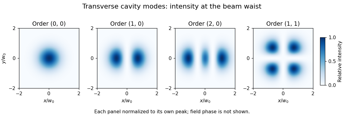
A transverse optical cavity mode is a resonant field pattern across the direction of propagation in an optical cavity. After propagation and reflection through a round trip, the mode reproduces its transverse shape up to a complex amplitude factor. Longitudinal order counts axial phase cycles; transverse order describes the pattern across the beam. Different transverse patterns can resonate at the same frequency, as in confocal transverse-mode degeneracy.

In an ideal paraxial cavity with suitable spherical mirrors, a Cartesian Hermite-Gaussian optical mode at its waist has field proportional towhere $H_m,H_n$ are Hermite polynomials, $m,n$ are nonnegative integers, and $w_0$ is the beam waist radius. The intensity is proportional to $|u_{mn}{|}^2$, not to the signed field. The primary photonics notes give these transverse solutions, their phase advance and lower-order patterns.^[ref]

For $(m,n)=(0,0)$, the intensity is a single Gaussian beam spot. For $(1,0)$, $H_1(s)=2s$, so intensity is proportional to $x^2{e}^{-2(x^2+y^2)/w_0^2}$. It vanishes on $x=0$ and its two maxima occur at $x=\pm w_0/\sqrt{2}$, $y=0$. The two lobes have opposite field signs even though both have positive intensity. The $(1,1)$ pattern has two crossing nodal lines and four intensity lobes.

For an ideal empty two-mirror cavity of length $L$, set $g_i=1-L/R_i$. On the near-planar stable branch with $g_1,g_2>0$, the resonance frequencies areThe transverse contribution is a Gouy phase correction to the round-trip phase. Other branches require a consistent phase choice; the square root alone should not erase that choice. For an original example, $L=0.10\mathrm{m}$ and $R_1=R_2=0.20\mathrm{m}$ give $g_1=g_2=1/2$ and a one-order transverse spacing $c/(6L)\approx 499.65\mathrm{MHz}$ at fixed $q$. Modes with the same $m+n$ are degenerate in this ideal symmetric model.

A proposed observation scans cavity length while recording both transmission peaks and a camera image of the transmitted beam. Translating or tilting the incident beam changes its overlap with different transverse modes; matching the incident wavefront and width favors the fundamental mode. A transmission peak alone cannot identify the spatial pattern, and an intensity image alone does not recover its phase. Finite apertures, astigmatism and mirror imperfections alter losses and split ideal degeneracies; state the cavity geometry and imaging plane when comparing observations.

The operating pressure angle ${\alpha }_w$ is the gear pressure angle of an actual meshing pair at its mounted axis separation. For external spur gears with involute profiles, it is the angle between the gear line of action and the common tangent to the operating pitch circles. Changing the separation changes this angle even though the individual gear base circles remain fixed.^[ref]

Let the two base radii be $r_{b1},r_{b2}$ and the mounted axis separation be $a$. The right-triangle geometry of the gear line of action givesIf $a_0=r_1+r_2$ is the reference separation and both reference gear pressure angles equal $\alpha$, then $r_{bi}=r_i\cos \alpha$, henceThe gear reference circles and gear ratio remain unchanged by this mounting adjustment; the operating pitch circles expand or contract to fit $a$.

For example, reference radii $20\mathrm{mm}$ and $40\mathrm{mm}$ with $\alpha =20{}^{\circ }$ give $a_0=60\mathrm{mm}$. Mounting a compatible pair at $a=61\mathrm{mm}$ givesAt an imposed gear tangential force $100\mathrm{N}$, the associated gear separating force is about $41.30\mathrm{N}$, compared with $36.40\mathrm{N}$ at the reference angle. Holding torque instead of tangential load would additionally require using the changed operating radius.

The angle formula is only a geometric condition. Usable tooth flanks must still reach the contact region and maintain an adequate gear contact ratio; excessive separation can destroy useful contact. Likewise, the existence of a real inverse cosine does not establish that a proposed mounting has suitable backlash or mechanical strength.^[ref]

A mathematical glyph variant is an alternative ready-made glyph supplied for a mathematical shape at a different extent. In an OpenType MATH table, each MathGlyphVariantRecord pairs a glyph index with its advanceMeasurement along the extension direction.^[ref]

Consider an invented set of vertical variants with construction measurements 900, 1300 and 1800 font units. A selection policy seeking the smallest variant at least 1200 units tall chooses 1300; a target of 1700 chooses 1800. A target of 2000 exceeds the set and may need a mathematical glyph assembly if the font supplies suitable parts.

This discrete choice is useful for growing mathematical delimiters around tall expressions. The numbers are an explanatory selection example, not measurements of an installed computer font. A separately drawn taller glyph can change proportions without requiring every stroke to undergo the same uniform enlargement.

A mathematical glyph assembly constructs an extended mathematical shape from positioned glyph parts. An OpenType MATH table records each part's full advance and glyph connectors; extender parts may repeat, with overlaps joining neighbouring pieces.^[ref]

For an invented vertical assembly, take bottom, middle and top parts with advances 500, 400 and 500 font units. Give each joining connector length 150 and require at least 80 font units of overlap. Choosing overlaps of 100 is then allowed. Starting at zero puts the parts at offsets 0, 400 and 700, giving total extentRepeating the middle part once, with another 100-unit overlap, adds $400-100=300$ and gives extent 1500. These are construction measurements along the growth direction, not a claim about a particular font's ink bounds. Positioning the assembled shape relative to the text baseline remains a separate layout choice.

A mathematical font constant is a font-specific parameter used in mathematical typesetting. The MathConstants portion of an OpenType MATH table supplies distances, percentages and other parameters, including the Math axis offset and script scaling.^[ref]

For an invented distance example, suppose a computer font uses 1000 font units per em and specifies fractionRuleThickness as 40 font units. At 25 pixels per em, the ideal typeset fraction bar thickness isAt 50 pixels per em, the same stored value gives 2 pixels before rasterization adjustments. A percentage value such as 80, however, is a ratio and must not be converted as though it meant 80 font units.

Keeping the units explicit prevents plausible-looking scale errors. Suggested values in the specification guide font design; they are not universal dimensions shared by every computer font.

A quantum dynamical semigroup is a continuous family $({\Phi }_t{)}_{t\ge 0}$ of linear maps on density matrices satisfying ${\Phi }_0=I$ and ${\Phi }_{t+s}={\Phi }_t\circ {\Phi }_s$, with each map completely positive and trace preserving. The composition law expresses time-homogeneous evolution with no dependence on how the interval is divided.

In finite dimensions, continuity gives ${\Phi }_t=e^{t\mathcal{L}}$, whose generator has Lindblad equation form. For a qubit dephasing example,Off-diagonal decay factors multiply under composition, while populations stay fixed. The map is the mixture $(1+e^{-\gamma t})\rho /2+(1-e^{-\gamma t})Z\rho Z/2$, which verifies complete positivity. A semigroup need not have physical inverse maps at positive times: undoing this decay would generally amplify coherence beyond valid states.^[ref]