
Sheafification Created 2026-09-24 Updated 2026-09-24
Sheafification associates a sheaf to a presheaf without changing its stalks and is universal among morphisms from that presheaf to sheaves.
Stalk of a sheaf Created 2026-09-24 Updated 2026-10-06
The stalk is the direct limit of over neighborhoods of . A morphism of sheaves is an isomorphism or forms an exact sequence exactly when it does so on every stalk.
Transgression Created 2026-09-24 Updated 2026-09-28
A transgression is a spectral-sequence differential from a fiber class on the vertical edge to a base class on the horizontal edge.
Harmonic series Created 2026-09-24 Updated 2026-10-14
The harmonic series is the positive seriesIts partial sums are the harmonic numbers . Although the individual terms tend to zero, grows without bound, so the harmonic series is not a convergent series. This is a basic warning against using the size of one term as a bound on all the terms still to come.
The growth is slow enough to be visually deceptive. The partial sums at are approximately . Adding ten times as many terms increases the accumulated total by roughly , rather than multiplying the total by ten. The telescoping series has similarly vanishing terms but approaches the finite sum one.
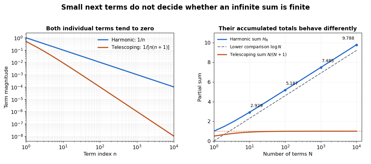

A short block argument proves the divergence without trusting a finite plot. For each integer , the block from through contains terms, each at least . ThereforeEvery doubling supplies at least another half, and arbitrarily many doublings are possible. A collection of tiny terms can still have a substantial combined contribution. See Jiří Lebl, Basic Analysis I, Example 2.5.11 for this grouping proof.
Integral comparison sharpens the growth estimate. Here denotes the natural logarithm. Since is a strictly decreasing function for positive , comparison of rectangles with the integral givesThus the divergence is logarithmic. The finer difference tends to the Euler--Mascheroni constant, approximately ; the harmonic number expansion supplies higher-order corrections. This turns the counterexample into a usable quantitative estimate of accumulated reciprocal contributions.
Euler's De progressionibus harmonicis observationes, written in 1734 and published in 1740, studies these sums beyond the yes-or-no question of convergence. Sections 2–3 compare long blocks to show continued growth, and later sections compare the sums with logarithms and calculate the constant offset. The [ref]
https://scholarlycommons.pacific.edu/euler-works/43/. Euler Archive record, E43
identifies the dates and original publication; [ref]https://download.uni-mainz.de/mathematik/Algebraische%20Geometrie/Euler-Kreis%20Mainz/E43.pdf. Alexander Aycock's translation of Euler's original paper
makes the calculations accessible. This is not a claim that Euler first discovered divergence: the paper's interest includes measuring how slowly a divergent sum grows. Partial sum Created 2026-09-24 Updated 2026-10-14
The th partial sum of a series with terms is the finite sum . It records the accumulated total after additions. The terms and their partial sums are different sequences: the terms of the harmonic series get small, while their partial sums grow without bound.
For the telescoping series with terms , the first three partial sums areBy contrast, the harmonic series gives , , and , where is the harmonic number. Computing more partial sums approximates an infinite sum only when a limit of a sequence exists, and the tail of a telescoping reciprocal series shows how an error estimate can certify the approximation.
Limit inferior Created 2026-09-24 Updated 2026-10-14
The limit inferior of a real sequence isallowing a value in the extended real number line. For a finite value , it has two complementary meanings: for every , all sufficiently late terms satisfy , while arbitrarily late terms satisfy . The first prevents persistent dips below ; the second prevents any larger number from being the true lower edge.
For , the lower bounds in limit inferior and limit superior approach . Every late term eventually exceeds , and the subsequence at odd integers comes arbitrarily close to . For , the lower bound of every infinite tail of a sequence is already zero, although no term equals zero. Thus a limit inferior need not be the minimum of any tail.
Limit superior Created 2026-09-24 Updated 2026-10-14
The limit superior of a real sequence isallowing a value in the extended real number line. For a finite value , every gives an eventual upper bound , while arbitrarily late terms still satisfy . The second condition concerns recurrence at arbitrarily large indices, not the fraction of indices where a large value occurs.
In limit inferior and limit superior, has limit superior one because its positive branch approaches one from above and all later values eventually stay below . Changing any finite number of terms leaves the limit superior unchanged: once the tail of a sequence begins beyond those positions, all its suprema are the same as before. The sparse peaks can determine a limit superior example shows that even a set of peak indices with zero natural density can decide the upper long-run edge.
Monotone sequence Created 2026-09-24 Updated 2026-10-14
A monotone sequence has one of these directions for every index. Here increasing means nondecreasing and decreasing means nonincreasing: equal successive terms are allowed. Strict increase would require at every step, and strict decrease would require . A constant sequence is both increasing and decreasing. These conventions are those of Basic Analysis: Introduction to Real Analysis, Volume I by Jiří Lebl (§2.1.1, Definition 2.1.9).
For , the sequence increases toward one, while decreases toward one. Repeating each term gives the still increasing sequence . Plateaus do not obstruct the bounded monotone sequence theorem. Checking the sign of is often the simplest way to verify a direction; finding an upper bound or lower bound is a separate task.
Bounded sequence Created 2026-09-24 Updated 2026-09-29
Laguerre differential operator on polynomials Created 2026-09-24 Updated 2026-09-24
On polynomials with weighted inner productthe operatoris self-adjoint because . Its eigenvalues on polynomials of degree at most are ; its eigenvectors are scalar multiples of the Laguerre polynomials.
Finite-dimensional spectral theorem Created 2026-09-24 Updated 2026-10-14
Every self-adjoint operator on a finite-dimensional real or complex inner product space has an orthonormal eigenbasis, and all its eigenvalues are real. In orthonormal coordinates, a real symmetric matrix has the form , with an orthogonal matrix and a real diagonal matrix. A complex Hermitian matrix instead has , with a unitary matrix and its conjugate transpose. These are the self-adjoint cases of the spectral theorem; Axler gives the real and complex finite-dimensional statements in Section 7B.[ref]
https://linear.axler.net/LADR4e.pdf. Sheldon Axler, Linear Algebra Done Right, fourth edition, Section 7B, Theorems 7.29 and 7.31; accessed 2026-10-11
An orthonormal eigenbasis turns a seemingly coupled linear map into independent scalar multiplications while preserving lengths and angles. If and , thenThe last identity removes every cross term from the quadratic form. The eigenvalues tell us whether it is positive, negative, or mixed in sign, and the eigenvectors identify the corresponding directions. This connects positive-definite matrices, quadratic forms, and the Hermitian Rayleigh quotient range.
For a fully computed example, takeDirect multiplication gives and . Their dot product is zero and each has norm one. ThusWriting changes into . Its level set is therefore an ellipse with semiaxis lengths and , along and . The coordinates change, but the ellipse does not: orthogonal diagonalization reveals its existing geometry.
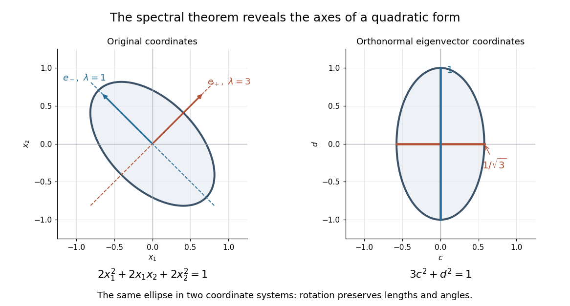
An orthonormal eigenbasis removes the cross term from a quadratic form and reveals the axes of its ellipse
. Details. 
For distinct eigenvalues, orthogonality follows at once from self-adjointness: . Within a repeated eigenspace, choose an orthonormal basis; arbitrarily chosen eigenvectors of the same eigenvalue need not be orthogonal. One outline of the full argument finds an eigenvector, observes that its orthogonal complement is invariant, and repeats in that smaller space. Merely having real eigenvalues is weaker: has two real eigenvalues, but its eigenvectors and are not orthogonal.
Fundamental group after attaching a 2-cell Created 2026-09-24 Updated 2026-09-24
Fundamental group after attaching a Möbius band Created 2026-09-24 Updated 2026-09-24
Generation of a fundamental group by two open sets Created 2026-09-24 Updated 2026-09-24
If , the sets , and their intersection are path-connected, and the base point lies in the intersection, then is generated by the images of and . Subdivide each loop into arcs lying in cover members and join every transition point to the base point within the intersection; the inserted paths telescope.
Amalgamated free product Created 2026-09-24 Updated 2026-10-03
Given homomorphisms and , the amalgamated free product comes with homomorphisms from and that agree on . It is universal with this property: every compatible pair of homomorphisms and factors uniquely through .
Seifert form Created 2026-09-24 Updated 2026-09-24
For oriented curves on a Seifert surface, the Seifert form iswhere is a positive normal push-off of .
Seifert genus Created 2026-09-24 Updated 2026-10-14
Fundamental forms of a graph surface Created 2026-09-24 Updated 2026-09-24
Mean curvature Created 2026-09-24 Updated 2026-10-14
Mean curvature measures the average signed bending of a smooth surface. Unlike Gaussian curvature, it adds the two principal curvatures rather than multiplying them. A circular cylinder therefore has nonzero mean curvature despite zero Gaussian curvature, whereas a catenoid has zero mean curvature despite negative Gaussian curvature. The cancellation on a catenoid explains how a curved minimal surface can be stationary for surface area.
Choose a unit normal and the shape operator , as in the second fundamental form convention . For a smooth surface in Euclidean space of dimension three, define the signed scalar mean curvature byHere are the coefficients of the first fundamental form, and those of the second fundamental form. The factor makes an average; the scalar trace convention instead calls the mean curvature. Authors who use reverse both signs. A formula involving mean curvature is therefore incomplete unless its shape operator, unit normal, and averaging convention are specified.
In orientation reversal of surface curvature, both principal curvatures and change sign, while Gaussian curvature and the mean curvature vector do not. The units of mean curvature are inverse length, compared with inverse squared length for Gaussian curvature. The distinction matters in soap film pressure balance: pressure couples to the sum of the signed principal curvatures.
Gaussian curvature Created 2026-09-24 Updated 2026-10-14
Rolling a sheet into a circular cylinder bends it without changing its internal lengths and angles. Fitting that same sheet smoothly onto a sphere requires distortion of its first fundamental form. Gaussian curvature distinguishes these situations: it measures the intrinsic curvature of a smooth surface, even though its simplest definition uses how the surface bends in Euclidean space.
The Gaussian curvature at a point is the determinant of the shape operator, or the product of the two principal curvatures:Here is the first fundamental form and is the second fundamental form, with . Regularity makes . Reversing the unit normal negates and both principal curvatures, leaving Gaussian curvature unchanged. [ref]
https://ghomi.math.gatech.edu/Classes/Math497C/LectureNotes9.pdf. Ghomi, Lecture Notes 9, §2.2: determinant formula and independence of normal choice
The sign describes bending at the point: positive Gaussian curvature means the principal curvatures have the same nonzero sign, as at an elliptic point; negative Gaussian curvature means opposite signs, as on a saddle; zero Gaussian curvature means at least one principal curvature vanishes. Zero Gaussian curvature at a single point does not imply that a neighborhood is a plane. [ref]
https://ghomi.math.gatech.edu/Classes/Math497C/LectureNotes10.pdf. Ghomi, Lecture Notes 10, §2.3.1: the sign of Gaussian curvature
Four worked models make the signs concrete:
- On a plane, the unit normal is constant, so the shape operator is zero and .
- On a sphere of radius , the outward unit normal gives . Thus , , and .
- On the lateral surface of a circular cylinder of radius , the outward unit normal gives and . Hence but : there is extrinsic curvature despite intrinsic flatness. The shape operator calculation above gives , , , so the determinant formula gives the same result.
- For the upward-oriented saddle with , the gradient vanishes at the origin. The fundamental forms of a graph surface therefore giveThe shape operator has eigenvalues , giving and . Away from the origin, Gaussian curvature of a graph surface gives ; the label applies only at the marked point.
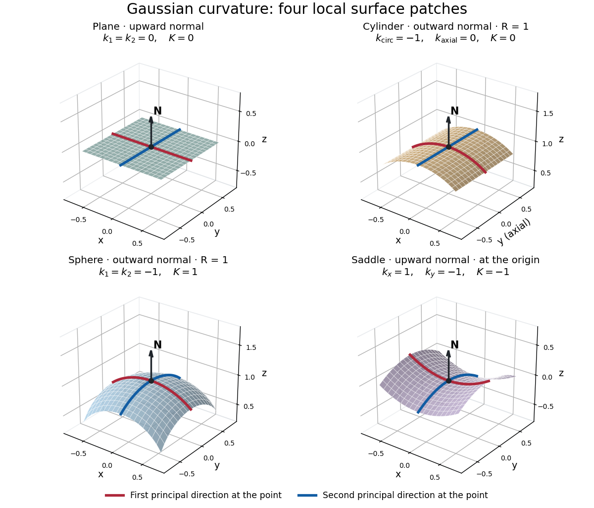
Plane, outward cylinder, outward sphere, and upward saddle compared by their principal curvatures and Gaussian curvature
. Details. 
The patches use a common length unit, with for the sphere and circular cylinder. The marked red and blue curves have principal directions at the black point; the arrow is the chosen unit normal. For physical lengths, principal curvature and mean curvature have units of inverse length, while Gaussian curvature has units of inverse squared length. Rescaling a surface by divides its principal curvatures by and its Gaussian curvature by . Writing the saddle as restores an explicit length scale: .
The Theorema Egregium says that Gaussian curvature depends only on the first fundamental form and its first two coordinate derivatives. A local isometry therefore preserves Gaussian curvature, even if the shape operator and the principal curvatures change. [ref]
https://ghomi.math.gatech.edu/Classes/Math497C/LectureNotes11.pdf. Ghomi, Lecture Notes 11, §2.5: Theorema Egregium
Here is the outline, rather than a full proof. The Gauss formula splits second derivatives of a parametric surface into tangential Christoffel symbols and the second fundamental form. The Christoffel symbols are determined by the first fundamental form and its first derivatives. Commuting the next partial derivatives gives the Gauss equation, which identifies with the intrinsic sectional curvature computed from the Riemann curvature tensor. Thus the apparently extrinsic product is determined by the Riemannian metric. [ref]
https://ghomi.math.gatech.edu/Classes/Math497C/LectureNotes12.pdf. Ghomi, Lecture Notes 12, §§2.6–2.7: Gauss formula and metric-based curvature
One can see the distinction directly by rolling a plane strip with coordinates into the circular cylinder . Both have , so the map is a local isometry, and is one-to-one on an open strip of width less than . Extending over all real numbers wraps around periodically; it does not give a global isometry between the entire plane and the entire circular cylinder. A nonempty open patch of a sphere cannot be flattened by a local isometry into a plane, because its Gaussian curvature cannot become zero. The obstruction concerns preservation of the first fundamental form, rather than a particular drawing or choice of seam.
There are unlisted articles, also show them or only show them.