
The beam splitter sends transmitted and reflected portions into perpendicular arms. Each mirror returns its beam to the splitter, where the two returning fields recombine towards the detector. A collimating lens provides approximately plane illumination. A compensating plate of the same glass thickness as the beam splitter can equalise the dispersive glass paths, which matters especially for broadband light.
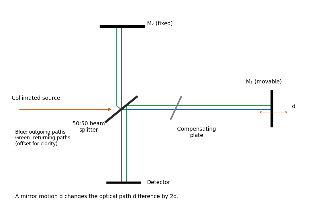
In division of amplitude, one incident beam is split into two or more parts at a partially reflecting interface; they follow distinct paths and are recombined. The Michelson interferometer and thin-film interference use this principle. In division of wavefront, spatially distinct parts of the same wavefront are selected and allowed to overlap, as in double-slit interference. Both require adequate optical coherence; wavefront division particularly exposes the need for spatial optical coherence between the selected regions.
For a rectangular slit centred at , the one-dimensional Fraunhofer diffraction integral isThe two equal apertures have centres at ; the glass subtracts their fields. ThereforeThis is phase-reversed double-slit diffraction: the narrow-slit interference factor is multiplied by the single-slit diffraction envelope. In the limit , the normalized envelope tends to one, recovering part (d).
The interference minima and envelope minima obey, respectively,Near the axis these are and envelope zeros . Here , so every envelope zero already coincides with an interference minimum. The envelope strongly reduces the outer fringes; its central value is nonzero, but the total intensity still vanishes at because the two fields cancel. The sketch uses the small-angle coordinate; the equations above specify the exact angular zeros.
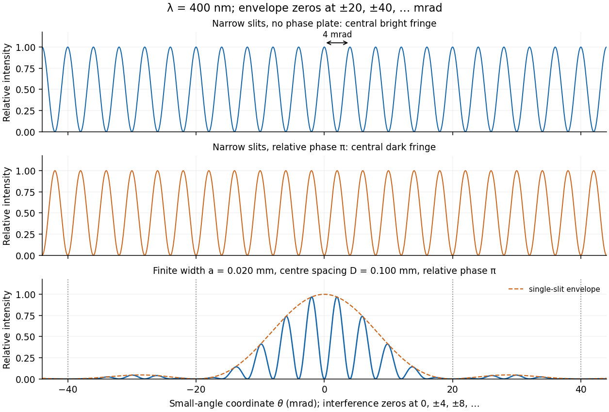
A relative phase changes the sign of one slit field. Their sum becomesThe central interference fringe is now dark. The maxima move to , while the minima occur at . Thus the pattern shifts by half a fringe, near the axis, but its angular fringe separation remains . This assumes the glass changes phase uniformly and introduces negligible absorption or beam deflection.
Represent equal narrow slits at by two contributions with equal complex amplitudes. In a direction the path difference is , soTherefore double-slit interference givesThe bright interference fringes satisfy , with a central maximum. In the small-angle region,Dark fringes lie halfway between bright ones. Exactly, spacing is uniform in , not in at large angles. The first panel of the pattern figure below shows the narrow-slit result.
Let the aperture occupy the plane, with coordinates and opening . Write for the incident scalar complex amplitude and for its dimensionless amplitude transmission, including any imposed phase. The observation point has transverse coordinates , corresponding to the PDF's , and axial distance . Also is the wavenumber and .
The Huygens-Fresnel principle expresses the propagated field, up to common prefactors and an approximately constant obliquity factor, asIn the paraxial approximation, expand the path asThe last term is negligible in the Fraunhofer diffraction limit, while the first two terms and are common across the aperture. Factoring them out leavesIt is the two-dimensional Fourier transform of the transmitted aperture field, evaluated at transverse wavevector . For appreciable observation angles the corresponding exact directional components are used rather than .
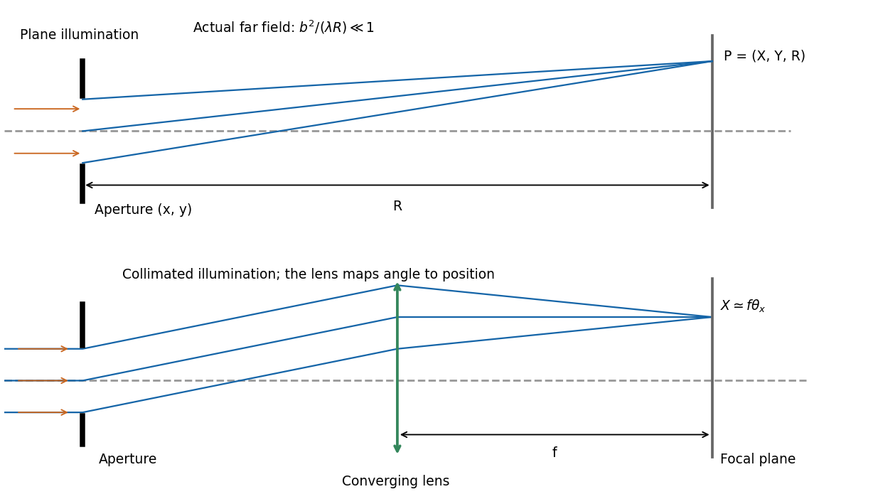
In Fraunhofer diffraction, the relative propagation phase across the aperture is linear in aperture coordinates. If is its largest transverse size, the neglected quadratic path term must be small: for an observer at distance ,For a finite-distance point source a distance away, also require if the illumination is to be treated as a plane wave. Numerical factors depend on whether is a radius or full width and on the permitted phase error; the condition expresses a small Fresnel number.
One can place both source and screen sufficiently far away, or collimate a point source with a lens and observe the aperture in the back focal plane of a second lens. In the latter arrangement rays of each outgoing direction focus at one point, with ; the lens removes the need for a physically distant screen. A laser beam approximately uniform across the aperture can supply the incident plane wave. The sketches distinguish an actual far field from its focal-plane equivalent.
The precise bandwidth depends on the output: this is the distinction between displacement and current bandwidths of a series RLC circuit. For current output, or voltage across the resistor, the electrical impedance givesThe half-power points satisfy . Their positive roots areChanging capacitance shifts the centre without changing this absolute width. For the charge response in part (d), the exact half-height points instead obeywhen both exist their separation only approaches at large quality factor. Therefore the printed capacitance-independence claim is exact for current or resistor-voltage output and an approximation for the preceding charge resonance.
For a narrow band-pass filter, use current or resistor-voltage output and make small, counting source, load and inductor losses in the total electrical resistance. Increase ; if a specified centre frequency is to remain fixed, adjust with to keep fixed. Capacitor-voltage output alone is not a band-pass response because it has a nonzero DC limit.
The capacitor-charge complex amplitude isFor fixed driving-voltage amplitude, maximizing minimizesDifferentiate:The positive-frequency minimum therefore hasThis is the resonance of charge, or capacitor voltage. If the stated inequality fails, their maximum is at zero frequency, and no positive displacement-resonance peak exists. The electric current has the additional factor , and instead peaks exactly at for every .
The original diagram is a series RLC circuit, so the same electric current passes through all three elements. Choose capacitor electric charge positive on the plate into which positive enters. Kirchhoff's voltage law givesDividing by inductance givesThe correspondence to the forced harmonic oscillator is , , , and . The stored energy is ; its balance is , confirming the damping sign.
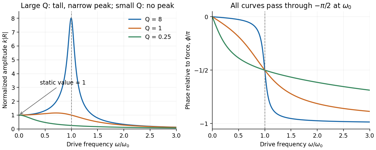
For the steady response of a forced harmonic oscillator, write and use the same complex amplitude convention for the driving force. Substitution givesThus the response magnitude and displacement phase relative to the force areThe phase goes from at low frequency, through at , towards at high frequency. The static magnitude is , while the high-frequency magnitude is approximately .
Define the quality factor by . If , the displacement peak occurs at ; for the magnitude decreases monotonically from its static value. For there is a tall narrow peak close to , of height approximately and width approximately . At very small the resonant peak disappears and the response is broad. The plotted functions are normalized as , at fixed .
Substituting into the damped harmonic oscillator equation givesFor nonnegative viscous damping, the cases areThe PDF's request to express these conditions in terms of is dimensionally inconsistent with its definition : already has units . With the unnormalised equation , the equivalent comparisons are , or . Also is the undamped natural angular frequency, not in general the driven displacement peak.
Past exam of the physics A course of the University of Cambridge 2018 Paper 1 Section D D13 c Solution Created 2026-10-18 Updated 2026-10-20
Johnson-Nyquist noise is equilibrium electrical fluctuation caused by thermal agitation of charge carriers. A resistor can generate a fluctuating terminal voltage even when its mean current is zero. In the classical frequency range , the fluctuation-dissipation theorem relates this noise to dissipative resistance. The one-sided voltage power spectral density of an unloaded resistor isEquivalently its short-circuit current spectrum is . Over a flat bandwidth the rms voltage is . A real measurement instead integrates over positive frequency, with loading and the filter's effective noise bandwidth included. A flat spectrum does not imply an infinite physically measurable variance; the circuit and the quantum high-frequency regime limit the ideal white-noise model.
Cooling or narrowing the accepted bandwidth reduces thermal noise. Reducing resistance lowers its open-circuit voltage noise but raises its short-circuit current noise, so the appropriate choice depends on source impedance and amplifier loading. Thermal agitation is not a fluctuating externally applied voltage that can be removed by perfect shielding alone.
Shot noise arises from discrete transfer events. In the simplest shot noise counting model, equal charges arrive independently at constant rate . A gate of duration contains a Poisson number , with mean and variance . Therefore mean current is , and the averaged-current variance is . The corresponding one-sided low-frequency spectrum isfor a flat accepted bandwidth. Electron current has . Vacuum emission or photodetection can approximate independent arrivals; correlations in a conductor can suppress or enhance the fluctuations. Discreteness by itself does not guarantee Poisson statistics.
For a fixed mean current the ideal shot-noise formula is not proportional to temperature, whereas Johnson noise is. Increasing current raises absolute shot noise but lowers its fractional size, since . Both can appear approximately white within a useful frequency band, and independent noise powers add after referring them to a common measurement point. Their spectra must use the same convention: two-sided densities are half these one-sided values. A real low-current experiment can also contain amplifier noise, low-frequency drift and correlated transfer noise, so a mean current or resistance alone does not specify its complete noise budget.
A systematic error is a reproducible bias in the measurement model or procedure, such as a zero offset, incorrect gain, background contamination, misalignment, loading or temperature-dependent calibration. Repeating the same biased procedure more often reduces independent random scatter but does not remove the bias. An unknown correction also has a measurement uncertainty, even when the mechanism is systematic.
A simple instrument model is , with gain error , offset , drift and random noise . Comparison with calibrated standards at several input values separates an offset from a scale error and can test nonlinearity. Use standards that cover the operating range, verify units and reference values, and propagate uncertainty in the standards into the corrected result. Calibration changes the model; it does not make the corrected measurement exact.
A blank or source-off measurement estimates additive background. For independent source-plus-background count in time and background count in time , the net-rate estimate and its counting variance areSubtracting a measured background removes its estimated mean, not its fluctuations or its uncertainty. A long background exposure can reduce the latter, while drifting backgrounds require monitoring or a joint model.
Reversal can distinguish a wanted signal from an unchanged offset. For example, and give when the thermoelectric offset is stable between readings. Interchanging sample and reference, reversing field direction or reversing an apparatus orientation can similarly expose sign-dependent biases, but only if the wanted and unwanted contributions transform differently.
Track slow instrumental drift using frequent references, interleaved readings or an ABBA measurement sequence. Equal-time readings in the order A, B, B, A cancel a common linear drift in the difference estimator . Nonlinear drift or unequal sample conditions can survive. Randomizing run order helps prevent a time drift from imitating dependence on a controlled experimental variable.
Control physical couplings directly: stabilize temperature, minimize gradients, shield unwanted fields, align geometry, and use high input impedance when loading is the concern. Differential and bridge measurements suppress common changes when their channels are well matched. Varying an apparatus parameter or using an independent method can reveal an unsuspected bias. Report residual corrections, their uncertainties and correlations; adding more identical readings cannot justify discarding a shared calibration uncertainty.
Bayes' theorem updates prior knowledge using the likelihood of new observations. For alternative hypotheses ,The prior describes information before the data ; is the sampling likelihood, and the posterior describes the updated probabilities. Posterior odds equal prior odds times the likelihood ratio. A likelihood is a probability model for data at specified parameters, not automatically a normalized probability distribution over those parameters.
For a continuous parameter , the same rule uses densities: . Priors can encode positivity, physical limits, previous independent measurements or calibration knowledge. Their parameterization matters: a density uniform in a rate is not uniform in its logarithm. Proper priors make model evidences well defined; an arbitrary normalization in an improper prior is especially problematic for comparing models.
A counting example uses Poisson-gamma conjugacy. If a detector registers events in exposure with constant rate , . A gamma prior with shape and rate parameter , , givesThe posterior mean combines the prior rate with the observed rate , weighted by the prior and actual exposures. The parameters must use a consistent shape-rate convention. Small counts can leave substantial prior sensitivity; abundant informative data usually reduce it for regular identifiable models.
Independent old data can become the prior for a new experiment, giving the same result as joint updating under a consistent model. The new data must not also have been used to construct that prior, or the evidence is counted twice. A credible interval has a specified posterior probability under the chosen model and prior; this interpretation differs from repeated-sampling coverage of a confidence interval. Predictions for a future observation average its sampling distribution over the posterior, incorporating parameter uncertainty. Prior sensitivity checks and a defensible likelihood are therefore part of the inference, rather than Bayes' theorem itself supplying missing physical knowledge.
Introduce an additive background rate , from ambient radiation, detector dark counts or another weakly attenuated contribution. If denotes the unattenuated signal alone, the attenuation count model with an additive background isIt approaches a nonzero constant as the transmitted signal becomes small. The source-off background should ideally be measured in a separate long exposure and its uncertainty included in the fit; otherwise estimate jointly using a Poisson count likelihood.
There is a normalization detail: the given was itself obtained from an count measurement. If that measurement included the same background, then it measures , and the attenuation fit normalized to a total reference rate isWriting instead treats as a background-subtracted signal calibration. The difference is small here because the background is a few counts per second while is about two thousand, but the distinction prevents double-counting background. The last three observations alone do not give an exact value of , because residual transmitted signal and sizeable counting fluctuations remain.
For a candidate attenuation coefficient, the one-second expected count is . The model predictions areUse first the conservative signal-dominated range , where the count approximation is reliable and background is a small correction. Using the estimated errors from part (c), the weighted residual statistic isIt gives . Since both candidates are fixed and was calibrated independently, neither was fitted to these four counts: the approximate reference has , not three. The upper-tail probabilities are approximately and , respectively. Thus is compatible with the scatter, whereas is disfavored at the usual level in this approximate test.
A Pearson chi-squared statistic, using model variances instead of estimated observed variances, gives the same preference:Including the fifth point also leaves the decision unchanged: the estimated-error statistics are and on five degrees of freedom, with approximate upper-tail probabilities and ; the Pearson statistics are and . HenceThe small uncertainty in contributes correlated prediction uncertainty, as in chi-squared comparison of a calibrated attenuation model, but is negligible compared with the one-second counting errors here. Choosing the test range after inspecting the observations limits a strict interpretation of its nominal significance; the numerical comparison and its stated range are the relevant evidence.
If all eight observations are inserted into the estimated-error formula, the totals are and . Their nominal eight-degree-of-freedom calibration is unreliable because the final expected counts are much smaller than one for some predictions. In fact the full-range Pearson statistics are and , exposing the late excess much more strongly. The full Poisson deviance values are and , again favoring but signaling that a background-free exponential is inadequate over the complete range. These sparse-count comparisons should not be used to claim that either unmodified model explains all eight measurements.
Assume independent radioactive detections with negligible dead-time loss, so accumulated counts have a Poisson distribution. The reference measurement has total count over . Since a Poisson count has variance equal to its mean, the rate uncertainty isIts relative uncertainty is , or . For each one-second measurement, , giving the estimated count and rate uncertaintiesin counts, numerically the same in counts per second for these one-second exposures. Their fractional uncertainties range from about at the first sheet to – for the smallest counts. The long, high-rate reference is therefore much more precise. These are statistical errors; a longer exposure does not automatically remove calibration errors, source drift or background bias.
An exponential count rate appears as a straight line on a semilogarithmic plot:The early points decrease by roughly a factor per added sheet. Keeping the supplied fixed, a simple unweighted straight-line estimate from the first four logarithms isso the early trend is consistent with near one. This logarithmic estimate is illustrative; the final statistical comparison should use the count uncertainties rather than treating the logarithms as equally precise.
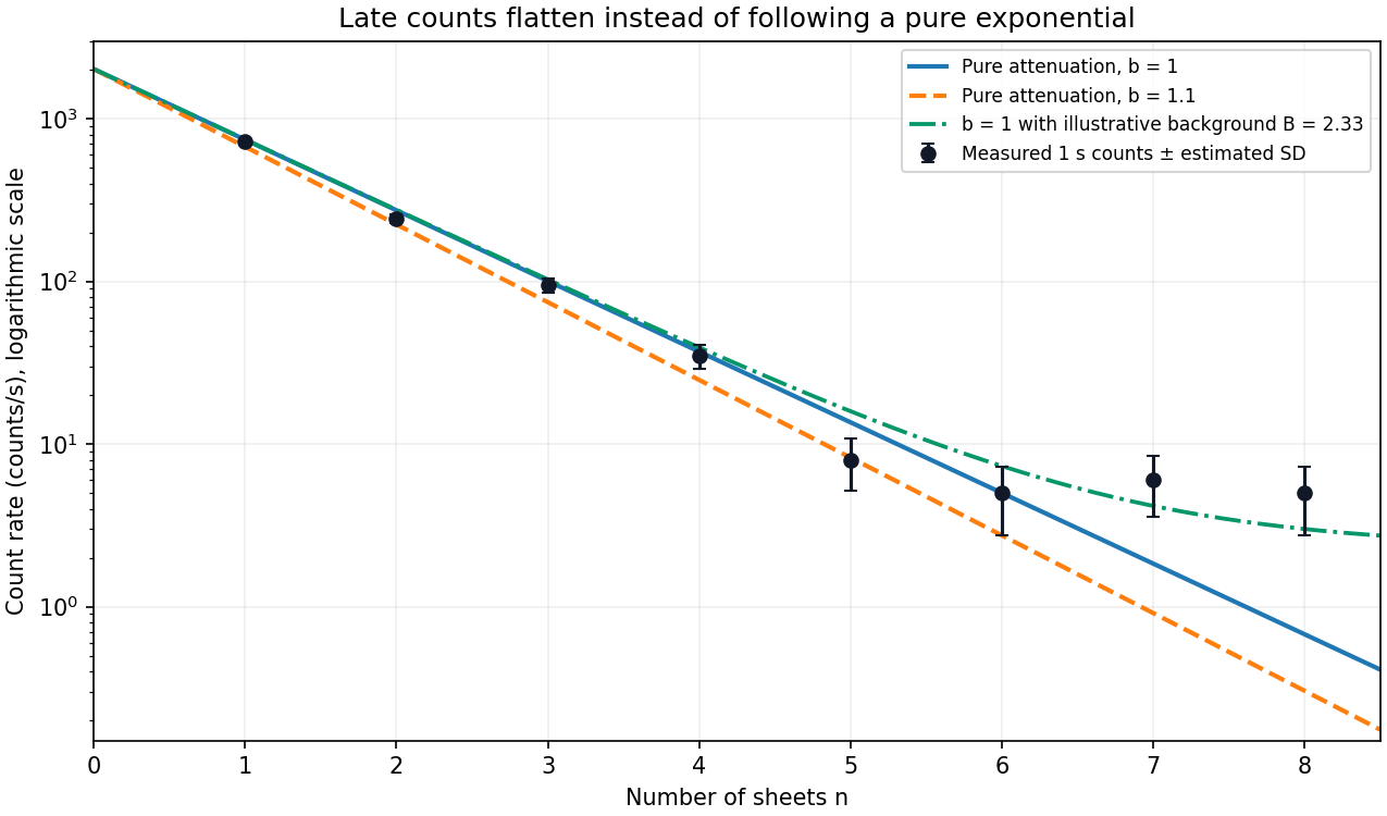


The pure exponential gives a useful approximate description through about the first four or five sheets. The first four observations are the clean high-count range; the fifth remains compatible with within its counting scatter. At the measurements are roughly constant at a few counts per second, so a single straight line no longer describes the whole pattern. Agreement of the sixth point with one exponential prediction by itself does not remove the systematic late flattening. There is no sharply determined physical cutoff from eight noisy measurements; the range used for a formal test should be stated explicitly.
A chi-squared test compares residuals with the random scatter predicted by a model. For independent measurements with known Gaussian standard deviations and predictions , formIf the mean model and error assumptions are correct, a full-rank linear fit of parameters gives a chi-squared distribution with statistical degrees of freedom. With a fully specified prediction and no fitted parameters, . Nonlinear fits usually make this an approximation. Independent external calibration is not the same as fitting a parameter to these test data.
Under the reference distribution, the mean statistic is and its variance is . The upper-tail p-value quantifies how unusual a discrepancy at least this large would be under the assumed model. A small value suggests model failure or incorrect uncertainties; it is not the probability that the model is true. An unusually small statistic can also reveal inflated uncertainties or correlations. A rejection threshold should be specified in advance.
For independent Poisson distribution counts, the model variance is its expected count . The Pearson chi-squared statistic is . The estimated-error alternative is common for large counts but can differ substantially when counts are small. In that regime the Poisson deviance or a direct likelihood calculation is preferable, with simulation if an accurately calibrated goodness-of-fit probability is required.
There are unlisted articles, also show them or only show them.