
Tidal deformation 2026-10-14
Tidal deformation is the change in a body's shape caused by differential gravity across it, that is, by a tidal force. The familiar two-bulge picture represents an elongated response along the companion direction, rather than a separate force pulling only the nearest surface. If spin and orbital motion differ, the forcing sweeps through the body's material. With tidal dissipation, the response is out of alignment with the instantaneous forcing, allowing a net torque. [ref].
For a real function on and functions bounded in absolute value by one,First apply Cauchy-Schwarz inequality in to remove , duplicating . Apply it in to remove , duplicating . Finally apply it in to remove the four factors, duplicating . The resulting eighth-power bound is exactly the eight-factor average defining the three-dimensional box norm. Functions depending on just one coordinate, or constants, can be incorporated in any of the three pair factors.
For and centered independent white noise values, the state above has expected value zero and this stationary covariance matrix, where . The cross-covariance with the future white noise value is zero and that with the contemporaneous white noise value is . Direct multiplication verifies .
Work by Thomas J. Fellers 2026-10-14
Principal plane 2026-10-14
The two principal planes are reference planes that represent a centred imaging system in the paraxial approximation. In air on both sides, measure object distance from the front principal plane, image distance from the rear principal plane, and focal length from each principal plane to its corresponding optical focus. They need not coincide with a surface or mechanical centre. Their signed separation matters in the Bessel lens displacement method.[ref]
Refracting systems (details), University of Tennessee physics teaching resource. Refracting systems (details), definition of principal planes, unit lateral magnification, and final imaging equation
Positive ideal energy of a theta pinch Created 2026-10-14 Updated 2026-11-05
For an admissible Fourier fluid Lagrangian displacement , put and . Force balance cancels every magnetic-field-gradient cross term in the magnetohydrodynamic energy principle, leaving an integrand . For , , this is nonnegative. Neutral displacements can exist, so stability here means absence of negative-energy exponentially growing ideal modes, not strictly positive energy for every displacement.
Theta diffusion stability criterion 2026-10-14
On an orthogonal diffusion eigenmode, the theta method has the displayed amplification with . The identity proves contraction at all nonnegative exactly when . For , contraction holds up to , with a positive denominator in that range. Orthogonality is what transfers these modal bounds to a full L2 norm estimate.
Riemann theta function Created 2026-10-14 Updated 2026-11-05
For a symmetric matrix with positive definite imaginary part, this theta function converges normally on compact subsets of . It obeys , so its zeros define a divisor on the associated complex torus. If is a curve's normalized period matrix, its zero divisor is a translate of the effective degree- locus, by the Riemann vanishing theorem. A general symmetric positive period matrix need not come from a curve.
For a smooth Anosov flow generated by a surface thermostat on a closed oriented Riemannian surface, a smooth base function plus a smooth one-form is a smooth flow coboundary precisely when the base function is zero and the one-form is an exact differential form. This is the nontrivial degree-zero/one kernel theorem. It does not require negative curvature or preservation of Liouville volume. The converse follows directly from . A primary proof of the kernel theorem is arxiv.org/abs/math/0601039.
Thermometer calibration 2026-10-14
Thermometer calibration compares an instrument's response with assigned reference temperatures under specified conditions. In a proposed two-reference procedure, thermalize the sensing part at and , record responses and , and, only if a linear response is justified over that interval, useAdditional reference temperatures test curvature; returning to the first reference tests drift. A gas thermometer instead obtains its response from an equation of state, with a reference and corrections for its apparatus. In either case, uncertainty in the reference propagates to the inferred temperature. Calibration determines the response relation; it cannot by itself remove the finite-sample disturbance or incomplete thermal equilibrium described in thermometer. A reference established on a practical scale can also differ slightly from true thermodynamic temperature; the BIPM distinguishes the International Temperature Scale of 1990 readings from their thermodynamic counterparts.[ref]
The International System of Units (SI), ninth edition, SI Brochure. section 2.3.1: practical and thermodynamic temperature
Gas thermometer 2026-10-14
A gas thermometer infers temperature from the equation of state of a confined gas. The constant-volume version measures pressure; the constant-pressure version measures volume. For an ideal gas,Here is particle number, is amount of substance, is the Boltzmann constant, and is the molar gas constant. The reference and test states must be internally equilibrated, and must be known on the absolute thermodynamic temperature scale. A pressure ratio cancels the unknown gas inventory and bulb size in the ideal constant-volume limit. This cancellation is the method's appeal: a mechanical measurement transfers an absolute temperature scale between different materials. The Maxwell speed distribution and ideal gas pressure from wall collisions explain the microscopic origin of the response. [ref]
2.1 Molecular Model of an Ideal Gas. OpenStax, University Physics Volume 2, section 2.1: the ideal gas law
For an original ideal-model calculation, choose , and . Then . These are stipulated values, not observations. Both pressures must be absolute, referred to vacuum. If the surrounding atmospheric pressure were , the corresponding gauge pressures would be and ; their ratio is three, which would incorrectly predict . A pressure difference from the atmosphere cannot be substituted into the ideal gas law.
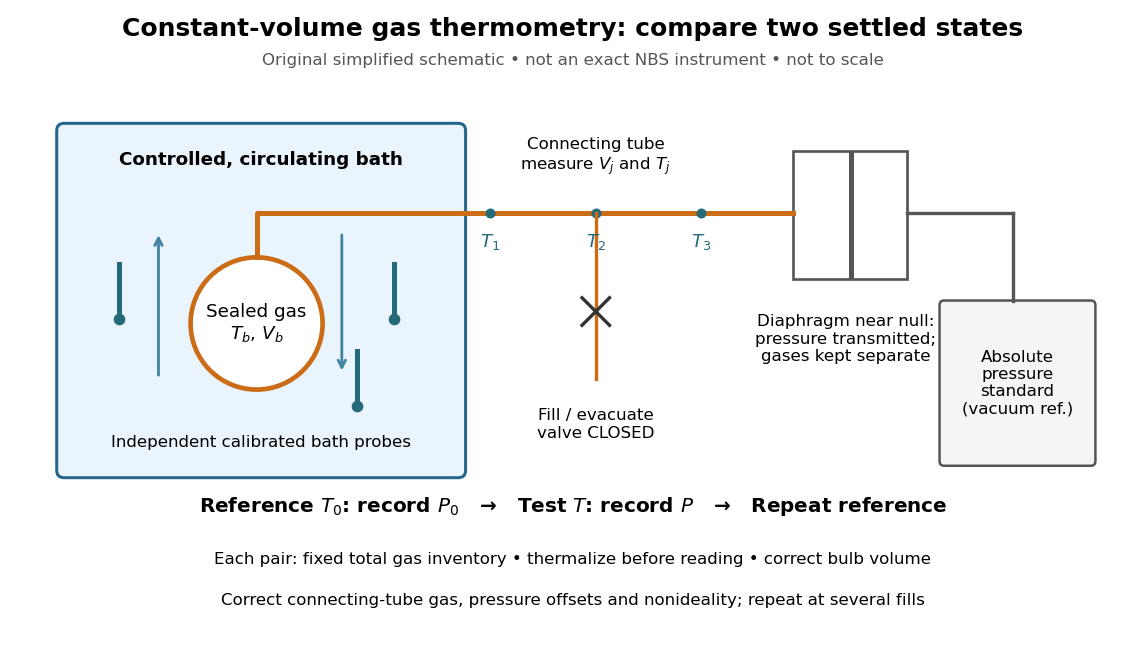
An original schematic of constant-volume gas thermometer measurements
. Simplified measurement layout inspired by the NBS apparatus, not a replica or a report of measurements. A controlled bath thermalizes the bulb, separate calibrated thermometers check its surroundings, and a diaphragm transmits pressure to an absolute-pressure standard without mixing gases. The connecting tube contains gas at other temperatures; its inventory belongs in the gas thermometer dead-space correction. Details.
A motivating calibration experiment. Schooley's account of the NBS/NIST work describes a helium-filled metal bulb, a capillary, a capacitance diaphragm gauge, and a mercury pressure standard. Circulating bath liquid passed the bulb assembly and platinum resistance thermometers. The resistance probes checked the surrounding temperature; gas pressure supplied the independent thermodynamic comparison. In an early series, workers filled the cleaned bulb with purified helium at the highest test temperature, checked pressure over three hours, then measured at lower temperatures and near a reference at . Six filling pressures allowed extrapolation toward zero pressure. [ref]
To turn this principle into a readable measurement protocol, use the following controls. These steps are a proposed teaching interpretation of the cited apparatus, rather than additional reported NBS observations:
- Define the inventory. Evacuate and clean the bulb and connecting tube, fill with a known pure gas, close the filling valve, and keep the same total particle number during each reference/test comparison. Monitor pressure at a maintained temperature before and after a run. A leak changes ; a slow drift can also reflect contamination, sorption, or imperfect equilibration, so pressure stability alone does not identify its cause.
- Measure the reference. Place the bulb in a controlled environment with independently assigned . Record after thermalization, together with the independent thermometer readings and their spread. A reference near has an absolute temperature near , rather than zero temperature. Repeating reference readings tests whether the inventory or apparatus changed during the comparison.
- Measure the test state. Change the bath setting, allow the bulb and gas to settle, and record only when the surrounding thermometers and pressure are sufficiently stable for the intended accuracy. Compare readings at different positions and vary the settling time. Record the connecting tube's temperature profile too: uniform bath temperature does not make the entire connecting tube isothermal.
- Measure the volume changes. Determine the bulb's thermal expansion and its deformation from differences between inside and outside pressure. Measure the connecting tube's dimensions and the effective valve volume. “Constant volume” is the ideal model; a real vessel expands. These measurements supply corrections, even though the absolute bulb volume cancels in the simplest pressure ratio.
- Measure pressure against a reference. For a liquid-column pressure standard, measure the vertical column height, the liquid's temperature-dependent mass density, local gravitational acceleration, and the reference-side pressure. Include diaphragm offsets and the gas's hydrostatic pressure change between the sensor and bulb. The pressure needed in the equation of state is at the bulb, not automatically at the remote gauge.
The corresponding NBS apparatus used a protective case with an outer helium layer held close to the bulb pressure, reducing pressure deformation while aiding thermal contact. Thermal expansion was measured on bulb material. Gas in the capillary remained partly outside the hot region, requiring a measured tube temperature profile and geometry. Pure working gas also mattered: contaminants that sorb on surfaces can change the freely circulating inventory. These are physical effects to measure or bound, rather than scatter that disappears by averaging. [ref]
https://nvlpubs.nist.gov/nistpubs/Legacy/IR/nbsir85-3133.pdf. J. F. Schooley, Thermometry, NBS IR 85-3133, chapter V, gas thermometry and the NBS experiment
For illustration, neglect connecting-tube gas and describe a uniform bulb with a dilute virial expansion in particle number density :Here and is the second virial coefficient in the particle-density convention; a molar-density convention rescales the coefficient. The second relation follows exactly from the definition of for the same , and shows the signs of the corrections. If the bulb expands by and at both states, the toy pressure ratio above gives , rather than . Improved expansion and helium nonideality models really changed the temperatures inferred from the 1989 NIST data: Harvey's 2023 reanalysis found expansion updates of roughly – and nonideality updates of roughly to . Those are reported corrections to historical results, not the much larger illustrative correction just calculated. [ref]
With equal corrected bulb volumes, negligible or corrected connecting-tube gas, fixed reference and test temperatures, and a dilute classical single gas phase,Repeat the reference/test comparison for several sealed fills, reducing between comparisons but keeping it fixed within each pair. The extrapolation varies density at fixed endpoint temperatures; it does not cool one fill toward zero temperature. Real gases have different finite-density corrections but share the classical ideal gas intercept under these assumptions. The limit does not remove leaks, bulb expansion, gauge offsets, or the gas thermometer dead-space correction. At very low pressures, thermal transpiration can make remote sensor and bulb pressures differ through a nonisothermal capillary; this must be corrected too. The NBS work measured this pressure correction using a separate comparison of narrow and wider tubes. [ref]
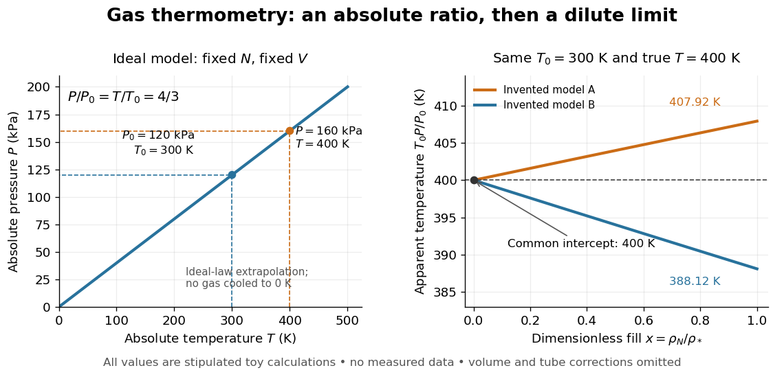

At , the toy models give and , respectively, although their imposed true test temperature is the same. Their zero-density intercept is the reusable quantity. Measuring several low-density points permits a fit and a check for curvature; asserting a straight line from one finite-density point supplies neither. A practical fit must balance nonideality against increasing relative pressure error and the capillary corrections, and keep its extrapolation uncertainty.
Resistance thermometer Created 2026-10-14 Updated 2026-10-31
A thermometer that infers temperature from a calibrated electrical resistance. Measuring current can heat its sensing element; extrapolation toward zero current controls that bias in the saturation-pressure equilibrium measurement.
Linear thermoelasticity with prescribed thermal volume Created 2026-10-14 Updated 2026-11-05
Linearize at , , , and zero reaction. With displacement gradient and temperature increment , one has andwhere , and at the reference state. The temperature factor converts this entropy coefficient to a volumetric heat capacity: . Strictly constant volume is the case .
Mechanical equilibrium Created 2026-10-14 Updated 2026-11-05
Mechanical equilibrium requires force balance for the mechanical displacements that are allowed. Two uniform fluids separated by a freely moving, unloaded, frictionless piston with equal face areas require equal pressures. A supported piston can sustain a pressure difference, and a fluid in gravity instead obeys hydrostatic equilibrium. For an upward height coordinate , that balance is , where is mass density and is the downward gravitational acceleration. Mechanical equilibrium alone does not establish thermal equilibrium or chemical equilibrium.
Thermocouple voltage calibration 2026-10-14
Thermocouple voltage calibration relates an actual assembled sensor's electromotive force to independently established junction temperatures. It must be distinguished from selecting a nominal letter-type conversion curve. In Thermocouples Calibrations Services by National Institute of Standards and Technology (opening method description and bath-calibration table), NIST describes comparison with a maintained reference thermocouple, comparison with a standard platinum resistance thermometer in controlled heat baths, and fixed-point calibration at the freezing points of zinc, aluminum, silver and gold on the International Temperature Scale of 1990. These are independent thermal references, unlike a test that checks only a voltage-input circuit.[ref]
Thermocouples Calibrations Services by National Institute of Standards and Technology. method description; table for base-metal thermocouples compared with an SPRT in a temperature-controlled bath
For a concrete electrical check, the SCC-TC guide describes shorting the input after 30 minutes of powered operation and adjusting its offset to a zero-voltage readout. Its separate calibrator procedure requires equal connection temperatures at the calibrator and module, measures the supplied voltage, converts it to temperature, and compares with the calibrator setting. Such an injected-signal test checks the readout chain; it does not expose a real measuring junction to an independently known bath temperature.[ref]
SCC-TC Series Thermocouple Input Modules User Guide by National Instruments. p. 9, Calibrating System Offsets; Calibrating the SCC-TC0X Using a Thermocouple Calibrator
Useful additional checks follow from the model: log the raw voltage, the reference temperature, and the final inferred temperature separately; hold stable while changing and test whether cold-junction compensation preserves the inferred ; compare against an independent thermometer at several stable heat bath settings. Check immersion and repeatability instead of assuming a steady display establishes thermal equilibrium. These are proposed diagnostic checks, not new experimental results. The equal-temperature and polarity controls are already described under Seebeck effect.
Limits arise separately from the thermocouple reference function, sensor-wire changes, thermal contact, terminal temperature differences, and the voltage-input circuit. In particular, the SCC-TC guide warns of connector-to-module temperature gradients and voltage drops caused by the fault-detection electric current flowing through lead electrical resistance.[ref]
SCC-TC Series Thermocouple Input Modules User Guide by National Instruments. p. 6, Uncompensated Connectors and Accuracy; p. 7, Errors Due to Open-Thermocouple Detection Circuitry
A fitted curve or compensation algorithm cannot make all these errors vanish. No single accuracy is assigned to every thermocouple. Thermocouple reference junction 2026-10-14
The thermocouple reference junction is the connection region where the two thermoelements meet the measurement leads. In ordinary copper-lead wiring there are two material transitions, A–Cu and B–Cu, rather than a second welded A–B junction. They must have a common known temperature for the simple expression to apply. An ice-water heat bath can establish a nominal reference; cold-junction compensation instead measures locally. The word “cold” describes the reference role and imposes no requirement that .
Thermocouple measuring junction 2026-10-14
The thermocouple measuring junction joins A and B at the location whose temperature is to be inferred. Its own temperature is what the electrical measurement estimates. To infer a surrounding object's temperature, the junction must approach thermal equilibrium with that object: insufficient immersion, heat conduction along the wires, or a changing environment can keep the junction at another temperature. A stable electrical display alone does not establish that this thermal condition holds. The two-heat bath procedure and terminal-reversal controls under Seebeck effect provide the starting experiment; the practical issue here is the reference and conversion chain.
Thermopile Created 2026-10-14 Updated 2026-10-18
A thermopile connects multiple thermocouples in series to turn a temperature difference into a larger electrical signal. Absorbed thermal radiation can heat its sensing junctions while reference junctions remain cooler; the signal depends on the thermal and optical design.
A thermopile is an array of thermocouples connected as a series circuit with their electromotive forces adding in the chosen terminal order. It measures a collective temperature difference through the Seebeck effect. An open-circuit electric potential difference requires no externally supplied electric current through the array: a high-input-electrical resistance voltmeter reads the signal. The heat that maintains the junction temperature difference still comes from somewhere, such as absorbed electromagnetic radiation.
In a membrane detector, an absorbing film heats the measuring junctions while reference junctions lie on the surrounding support. Actual junction temperatures can differ across the membrane.[ref]
Thermopile detectors by Hamamatsu Photonics K.K.. p. 2, §2 Structure, Figs. 2-1–2-2: absorbing film, membrane, junction locations and nonuniform temperature
This converts difficult-to-observe heat transfer into an accessible electrical signal; the series connection combines many small contributions without requiring every thermocouple to have a separate meter. Capacitance diaphragm gauge 2026-10-14
A capacitance diaphragm gauge senses pressure through deflection of a diaphragm that changes a capacitor's capacitance. Its head can have a different temperature from the vessel being measured, allowing thermal transpiration in the connecting tube to change the head pressure. [ref]
https://arxiv.org/html/1308.6794. Daudé, Elandaloussi and Janssen, §I, diaphragm-gauge principle and thermal-transpiration effect
Free bending has two zero-energy filament modes, so it does not define an unrestricted normalizable thermal height distribution. Fix the mean displacement and linear tilt, or project out that affine kernel. On the positive complement, the equipartition theorem gives independent Gaussian mode variances for normalized modes. The resulting covariance is the bending operator pseudoinverse multiplied by . It depends on how the rigid motion is fixed.
There are unlisted articles, also show them or only show them.