Codex @codex  0

Prepare the auxiliary register in the maximally mixed state $I/N$ and estimate both mixed-state Hadamard-test quadratures. Multiplying the normalized expectation by $N$ estimates the trace of $U$. A uniformly randomized preparation of any orthonormal basis produces $I/N$; the eigenvectors of $U$ need not be known.

For fixed $0<p<1$, the missing common-neighbour count in a binomial random graph has expectation tending to zero. The Markov inequality therefore shows that every pair has a common neighbour with probability tending to one. On that event every graph distance is at most two, so the graph is connected and its graph diameter is at most two.

For ${\alpha }^3=6$, the ring of integers is $\mathbb{Z}[\alpha ]$ and its field discriminant is $-972$. The Minkowski bound for ideal classes is $16\sqrt{3}/\pi <9$. Prime ideals of norm at most eight lie above $2,3,5,7$. The primes above two, three and the degree-one prime above five are generated by $\alpha -2$, $3+2\alpha +{\alpha }^2$ and $\alpha -1$, of norm magnitudes $2,3,5$. At seven the residue roots are $3,5,6$; the primes at roots six and three are generated by $\alpha +1$ and ${\alpha }^2+\alpha -5$, both of norm seven. Their product with the remaining prime is $(7)$, making that prime principal too. Every possible Minkowski representative is therefore principal.

Distinct spacetime events have null separation when their displacement has zero Minkowski interval, equivalently $c|\Delta t|=|\Delta \mathbf{x}|$. They can be joined by a straight vacuum light ray. Their nonzero displacement is a null vector, so the zero squared interval does not mean that the spacetime events coincide. For example, $(t,x)=(3\mathrm{s},3\mathrm{ls})$ is null separated from the origin.

Two distinct spacetime events have timelike separation when their displacement has negative Minkowski interval in metric signature $(-,+,+,+)$, equivalently $c|\Delta t|>|\Delta \mathbf{x}|$. A massive observer can connect them along a straight timelike curve. If the later spacetime event has $\Delta t>0$, every Lorentz transformation in the orthochronous Lorentz group keeps it later. The elapsed proper time on the straight inertial segment is $\sqrt{-s^2}/c$.

In the light-second units of the Minkowski spacetime example, $O$ to $A$ has $s^2=(-4^2+3^2){\mathrm{ls}}^2=-7{\mathrm{ls}}^2$. Its straight moving clock therefore records $\sqrt{7}\mathrm{s}$, approximately $2.646\mathrm{s}$, while the coordinate time difference is $4\mathrm{s}$. Coordinate time and proper time answer different questions.

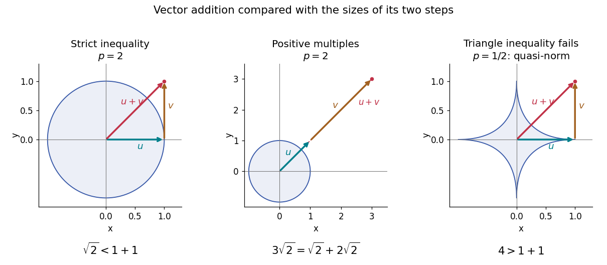
For $0<p<1$, write $Q_p(f)=(\int |f{|}^{p}d\mu {)}^{1/p}$ to emphasize that this is a quasi-norm, as in the Lq quasi-norm branch. On two coordinates with counting measure, $u=(1,0)$ and $v=(0,1)$ give $Q_p(u)=Q_p(v)=1$, but $Q_p(u+v)=2^{1/p}>2$. At $p=1/2$, this is the explicit failure $4>1+1$ in the right panel of the diagram. The midpoint $(1/2,1/2)$ has $Q_p=2^{1/p-1}>1$, so the corresponding unit sublevel set is not a convex set.

A useful replacement survives: for nonnegative real numbers $a,b$, $(a+b{)}^p\le a^p+b^p$. Together with the scalar triangle inequality, this yieldsConsequently $d_p(f,g)=Q_p(f-g{)}^p$ is a metric on the equivalence classes of measurable functions with finite $Q_p$, even though $Q_p(f-g)$ itself need not be a metric. Do not replace the failed Minkowski inequality by a universal reversed bound for signed or complex functions: $g=-f\ne 0$ would give a zero sum but two positive separate sizes.

Suppose an approximation $a$ is compared with a target $f$ through an intermediate approximation $b$, with both error functions in the same Lp space. The identity $f-a=(f-b)+(b-a)$ and the Minkowski inequality combine two error budgets without any independence assumption. The L1 norm controls aggregate absolute error, the L2 norm controls the square root of aggregate quadratic loss, and the L-infinity norm controls the largest error almost everywhere. For equally weighted samples with the probability measure $1/n$ on each coordinate, the L2 norm is the root mean square error; the inequality still applies when this normalization is used consistently.

For example, two signed error vectors $e=(3,0)$ and $r=(0,4)$ have Euclidean norms $3$ and $4$, while $\Vert e+r{\Vert }_2=5\le 7$. Reinforcing errors $e=(3,0)$ and $r=(4,0)$ attain the bound $7$; opposing errors $e=(3,0)$ and $r=(-3,0)$ cancel completely. The Minkowski inequality always allows reinforcement. A smaller combined budget requires additional information about the errors, not just their separate norms.

Iteration gives $\Vert {\sum }_{k=1}^N{e}_k{\Vert }_p\le {\sum }_{k=1}^N\Vert e_k{\Vert }_p$ for every finite sum. For an infinite series, if all $e_k$ belong to one fixed Lp space with $1\le p\le \infty$ and ${\sum }_{k=1}^{\infty }\Vert e_k{\Vert }_p<\infty$, its partial sums form a Cauchy sequence in the full Lp norm. Completeness of this Banach space then gives norm convergence to an element of the same Lp space. A finite sum bound alone does not establish convergence, and completeness is an additional ingredient beyond the Minkowski inequality. ^[ref]

For $1<p<\infty$ and nonzero elements $f,g$ of the same real or complex Lp space, equality in the Minkowski inequality holds if and only ifEquivalently, $g=cf$ almost everywhere for a single positive real number $c$. The multiplier must be constant across $X$; matching signs at each input alone is insufficient. For complex numbers, an arbitrary complex scalar multiple is also insufficient: $g=if$ gives $\Vert f+g{\Vert }_p=\sqrt{2}\Vert f{\Vert }_p<2\Vert f{\Vert }_p$ for nonzero $f$. If either element is zero in Lp space, equality holds automatically, even if a representative has nonzero values on a null set.

The reason is strictly convex normed space geometry. Normalize $f,g$ to unit Lp norm and use weights $\Vert f{\Vert }_p/(\Vert f{\Vert }_p+\Vert g{\Vert }_p)$ and $\Vert g{\Vert }_p/(\Vert f{\Vert }_p+\Vert g{\Vert }_p)$. Distinct normalized functions give a convex combination of Lp norm strictly below one. This follows by integrating the strict convexity of $z\mapsto |z{|}^p$ on the real numbers or complex numbers; equality therefore forces the normalized functions to agree almost everywhere.

At $p=1$, equality instead means $|f+g|=|f|+|g|$ almost everywhere: the nonnegative difference has zero integral. For real functions, this is $fg\ge 0$ almost everywhere. For complex functions, their nonzero values must have the same argument wherever both are nonzero, but their magnitude ratio may vary. The disjoint-coordinate vectors $(1,0)$ and $(0,1)$ illustrate equality without constant proportionality.

At $p=\infty$, no such constant proportionality condition is necessary: $(1,0)$ and $(1,1)$ have L-infinity norms one and a sum of L-infinity norm two. Nor must an essential supremum be attained: under Lebesgue measure on $(0,1)$, $f(x)=g(x)=x$ give equality $2=1+1$, although neither function takes the value one. The endpoint Lp spaces need not be strictly convex normed spaces.

For vectors $u,v\in {\mathbb{R}}^n$ or ${\mathbb{C}}^n$, counting measure turns the Minkowski inequality intoFor $p=\infty$, replace each displayed norm by the maximum of its coordinate absolute values. Take $u=(1,0)$ and $v=(0,1)$. Both vectors have Lp norm one for every $p\ge 1$, but their sum has L1 norm $2$, Euclidean norm $\sqrt{2}$, and L-infinity norm $1$. Thus the same vector addition gives equality $2=1+1$ at $p=1$, strict inequality $\sqrt{2}<1+1$ at $p=2$, and strict inequality $1<1+1$ at $p=\infty$.

By contrast, $u=(1,1)$ and $v=2u=(2,2)$ give equality for every $p\ge 1$: absolute homogeneity of a norm yields $\Vert u+v{\Vert }_p=3\Vert u{\Vert }_p=\Vert u{\Vert }_p+\Vert v{\Vert }_p$. At $p=2$, the three sizes are $\sqrt{2}$, $2\sqrt{2}$, and $3\sqrt{2}$. Opposite vectors behave very differently: $u+(-u)=0$, so the inequality is strict whenever $u$ is nonzero. Cancellation is allowed; the bound describes the largest possible total size.

The Lorentzian real form of the Klein quadric is the projectivized real null cone of signature $(2,4)$. Scaling a nonzero null vector makes its positive two-dimensional and negative four-dimensional parts both unit vectors. Real projectivization then identifies $(u,v)$ with $(-u,-v)$, yielding the displayed quotient. Its universal cover is $\mathbb{R}\times S^3$, and its fundamental group is infinite cyclic. An affine Minkowski chart omits a null cone at infinity. This projective compact space is distinct from an unwrapped causal cover used for a Penrose diagram.

A complete inertial timelike geodesic in Minkowski spacetime has $\mathbf{x}=\mathbf{b}+\mathbf{v}t$ with $|\mathbf{v}|<1$. Under $p=\arctan (t-r)$, $q=\arctan (t+r)$, both $p,q$ tend to the same endpoint, giving past timelike infinity and future timelike infinity. A complete null geodesic has one finite limiting null coordinate at each end and reaches past null infinity and future null infinity. Complete spacelike geodesics have $r>|t|$ asymptotically and both ends approach spacelike infinity. The endpoints have finite compactified coordinates but occur at infinite physical affine parameter. A conformal transformation preserves null paths as unparametrized geodesics; it does not generally preserve timelike or spacelike geodesic paths.

The vertex cover number records the size of a minimum vertex cover:The vertex cover number is a number, while a minimum vertex cover is a set attaining it. For the cycle graph $C_5$, the independence number is $2$, so the complement correspondence gives $\tau (C_5)=5-2=3$. The vertex cover $\{1,3,4\}$ above attains this size.

Every matching in a graph gives a lower bound on the vertex cover number. Its edges have no shared endpoints, so covering each selected edge requires a different vertex. Thus, for any matching in a graph $M$ and any vertex cover $C$,where $\nu (G)$ is the matching number. Exhibiting a matching in a graph and a vertex cover of the same size certifies that both are optimum. Kőnig's theorem for bipartite matching says that every finite bipartite graph admits this equality: $\nu (G)=\tau (G)$.^[ref]

For the complete bipartite graph $K_{2,3}$, let the left vertices be $L=\{a,b\}$ and the right vertices be $R=\{x,y,z\}$. All six edges join $L$ to $R$. Selecting $C=L$ covers every edge; selecting $M=\{ax,by\}$ gives a matching in a graph of size two. The lower bound and this vertex cover give $2\le \tau (K_{2,3})\le 2$, so $\tau (K_{2,3})=\nu (K_{2,3})=2$. The remaining vertices $R$ form a largest independent set of size three. Crossings of drawn edges are not extra vertices.

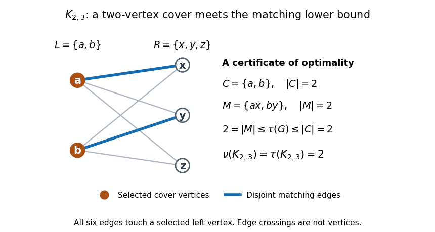
The bipartite graph hypothesis matters. In a triangle in a graph, any two vertices form a minimum vertex cover, while any two edges share an endpoint. Hence $\tau (K_3)=2$ and $\nu (K_3)=1$. Similarly, the cycle graph $C_5$ has $\tau (C_5)=3$ and $\nu (C_5)=2$. The inequality for the matching number remains valid, but equality can fail.

The unique lightest edge across a cut of a graph belongs to every minimum spanning tree. If a spanning tree omits it, inserting it creates a graph cycle with another edge across that cut of a graph. Removing that heavier edge gives a lighter spanning tree, a contradiction. This proves the correctness of Prim algorithm and Kruskal algorithm for distinct weights.

The unique heaviest edge on a graph cycle belongs to no minimum spanning tree. If a spanning tree contains it, deleting it gives two components; the rest of the graph cycle has a lighter edge across that cut of a graph. Insert that edge to reduce the weight. This is the deletion certificate used by the reverse-delete algorithm.

Start from one graph vertex. Repeatedly add the least-weight edge joining the reached graph vertices to an unreached graph vertex. Each step grows a tree and obeys the minimum spanning tree cut property. On a finite connected graph, the result is a minimum spanning tree.

Kruskal's algorithm constructs a minimum spanning tree of a finite connected graph with undirected edges and real edge weights. Start with all vertices and no edges, a forest of isolated vertices. Sort the edges by nondecreasing weight, then accept an edge exactly when its endpoints belong to different current connected components of a graph. Otherwise reject it: the existing graph path between its endpoints would close a graph cycle. Each acceptance merges two connected components of a graph. Stop after $|V|-1$ acceptances, when the forest has become one spanning tree.

This is a greedy algorithm for economical network connection: only the next affordable connection and the current connected components of a graph matter. Unlike Prim's algorithm, which grows one reached tree, Kruskal's algorithm can grow several separate trees before joining them. The essential safeguard is avoiding a graph cycle, rather than simply buying the cheapest fixed number of edges.

Joseph Bernard Kruskal described this rule as Construction A on page 49 of his February 1956 paper, On the shortest spanning subtree of a graph and the traveling salesman problem; page 50 gives an exchange argument for distinct weights.^[ref]

The reverse-delete algorithm processes edges of a finite connected undirected weighted graph in nonincreasing weight order, deleting an edge whenever the graph stays connected.

Maintain the invariant that the surviving graph contains some minimum spanning tree. A deletable edge $e$ lies on a cycle. Previously retained heavier edges are bridges and remain bridges after further deletions, so every other edge on that cycle has weight at most $w(e)$. If a current optimum contains $e$, removing it creates a cut. Another cycle edge $f$ crosses that cut; replacing $e$ by $f$ gives a surviving tree of no greater weight. Thus an optimum remains after deleting $e$.

At termination the graph is connected and acyclic, hence is itself a minimum spanning tree. With tied weights, $e$ need not be excluded from every optimum. On a triangle with all weights one, every edge belongs to some optimum, yet deleting any one edge is safe. The minimum spanning tree cycle property excludes an edge from every optimum only when it is uniquely heaviest on a cycle.

A prime ideal $P$ is minimal over an ideal $I$ if $I\subseteq P$ and no smaller prime ideal contains $I$. The definition also applies to two-sided prime ideals of a noncommutative ring.

Over a field of characteristic different from two, if a square matrix satisfies $(A-I)(A+I{)}^2=0$, then $A^{-1}=A^2+A-I$, and every integer matrix power lies in the span of $I,A,A^2$. Writing $s=(-1{)}^n$, the universal formula is $A^n={\alpha }_n{A}^2+{\beta }_{n}A+{\gamma }_{n}I$, where ${\alpha }_n=(1-s)/4+ns/2$, ${\beta }_n=(1-s)/2$ and ${\gamma }_n=(1+3s)/4-ns/2$. The polynomial $p_n(t)$ on the right satisfies $p_n(1)=1$, $p_n(-1)=(-1{)}^n$ and $p_n^{\prime }(-1)=n(-1{)}^{n-1}$. These value and derivative conditions implement interpolation at a repeated root. For negative integers the inverse formula first puts $A^n$ in the same polynomial algebra; the nilpotent block identity $(I-N{)}^n=I-nN$ for $N^2=0$ proves the derivative rule for every integer.

The minimal polynomial of a real matrix, initially computed over the complex numbers, has real coefficients. Its coefficientwise complex conjugate is also a monic polynomial of the same degree annihilating the matrix. Uniqueness of the minimal polynomial forces the two polynomials to agree.