
A real voltmeter has finite input electrical resistance ; a galvanometer also has a finite winding electrical resistance. Away from balance, its electric current changes both intermediate electric potentials. This is voltmeter loading when the detector is a voltmeter. Model the detector as a passive resistor, with no offset or injected electric current. Thévenin's theorem supplies the full response without pretending the connected bridge remains two independent voltage dividers.
With the detector removed, the equivalent source is . Replace the ideal supply by a wire to calculate the source electrical resistance seen between : nodes merge, making parallel and parallel. ConsequentlySince the attenuation factor is strictly positive for , the null remains . A smaller detector electrical resistance reduces the measured electric potential difference off balance but does not shift the ideal null. Its electric current sensitivity instead depends on ; detector gain and resolution also matter in deciding how closely a null can be located.
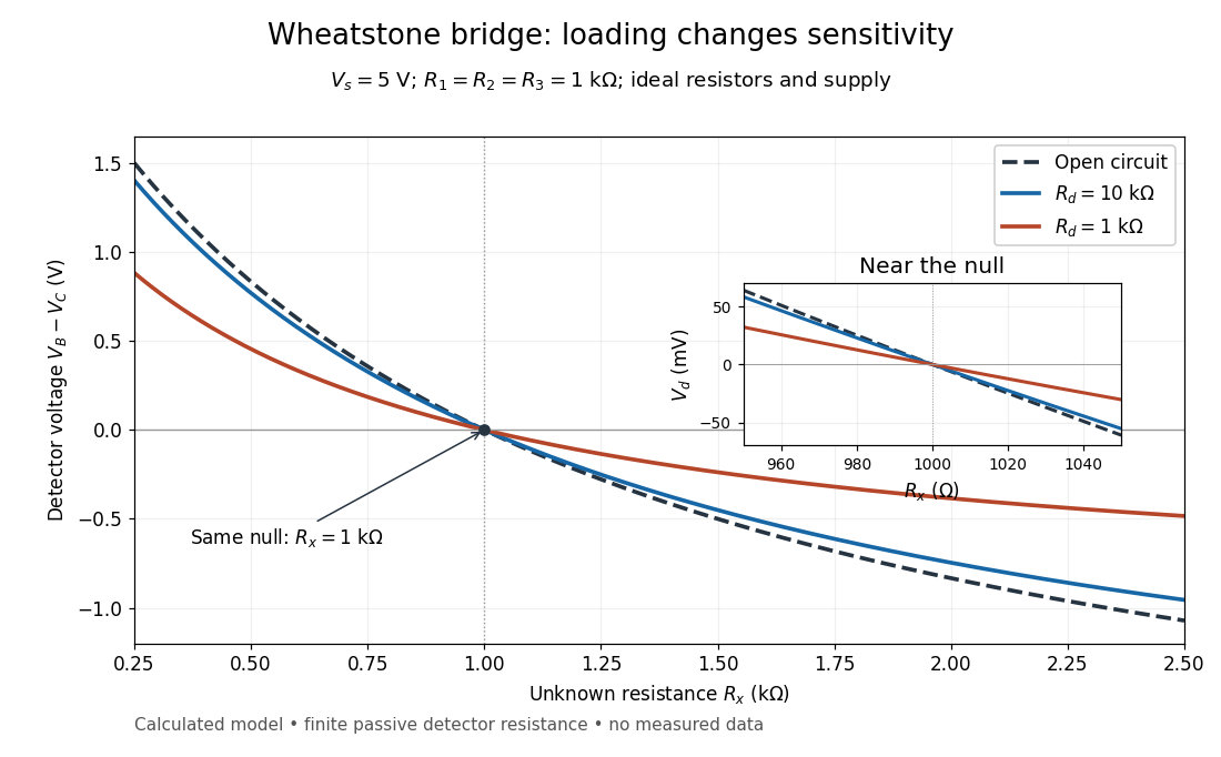
Finite detector resistance reduces bridge voltage sensitivity while preserving the null
. Calculated curves use and . All cross zero at ; the inset resolves their different slopes. These curves are a model, not measured data. Source. Details.
In the plotted example, gives and . A detector with instead reads . Using that loaded reading in the unloaded voltage divider formula would underestimate the deviation of from . Balancing the bridge avoids this particular systematic measurement error.
The local derivative makes the sensitivity explicit. For and , the first-order Taylor expansion isAt the plotted null, the open-circuit slope is , compared with for . Increasing the supply improves this ideal sensitivity but also increases Joule heating. A finite source electrical resistance requires recomputing ; the displayed parallel-pair expression assumes an ideal supply.
First disconnect the detector. Each side is a voltage divider. Ohm's law and Kirchhoff's voltage law give the open-circuit intermediate electric potentials and their difference:Setting this difference to zero and cross-multiplying givesThe balance compares ratios, not necessarily equal arm values or equal branch electric currents. At balance the detector carries no electric current, so Kirchhoff's current law again makes the electric current constant along each two-arm path.[ref]
For a worked null measurement, suppose and , and the detector null occurs at adjustable . ThenFor , both intermediate electric potentials are . The left branch carries and the right branch : the zero detector reading does not mean that the unknown carries no electric current. These are stipulated ideal values illustrating the calculation, not experimental observations.
A Western blot membrane is a thin protein-binding support that receives the separated pattern. It is a laboratory support, distinct from a cell membrane. Retaining proteins on its surface makes them accessible for Western blot antibody detection.
A known target-containing sample is a positive comparison for Western blot antibody detection. A matched sample with gene deletion supplies a negative comparison: disappearance of the proposed band supports the assignment, while a persisting band indicates binding unrelated to the deleted target. Deletion must actually remove the recognized protein; changes in other proteins can complicate the comparison. Omitting the primary antibody checks binding or background from the secondary antibody and detection reagents, but cannot exclude binding of the primary antibody to an unintended protein. Independent antibodies recognizing different epitopes add evidence. [ref]
Considerations when quantitating protein abundance by immunoblot by Alicia A. McDonough and others. McDonough and others, “Consider the Specificity of the Antibody for the Target”, Figure 2: positive tissue, knockout tissue and antibodies to different termini
A Western blot transfer control tests retention after Western blot transfer. Total-protein staining of the Western blot membrane can reveal uneven lanes or blank patches; staining the gel after transfer tests what remained behind. Transferred reference bands check selected positions, not recovery of every target. A pretransfer loading image alone cannot establish the amount retained on the receiving sheet.
A Western blot loading control estimates lane-to-lane sample differences. A reference protein, such as actin, must have stable abundance and detection responsive to amount. Equal saturated bands fail to establish equal loading. [ref]
Considerations when quantitating protein abundance by immunoblot by Alicia A. McDonough and others. McDonough and others, “Consider the Loading Controls”, Figure 4: sample doubling changes claudin detection but not the actin signal
A pH measurement becomes evidence for a weak acid chemical equilibrium when paired with a known analytical concentration and a calibrated glass electrode. For the pure-weak acid model, measured pH estimates only in the ideal thermodynamic activity approximation. Then , , , and . Require ; values outside that range signal inconsistent measurements or an inadequate model. Repeating this reconstruction across a dilution series tests whether one acid dissociation constant describes the data, rather than merely fitting one point.
The Analytical Sciences Digital Library's Potentiometric Titration of an Unknown Weak Monoprotic Acid provides a complementary acid-base titration experiment. Its apparatus includes a glass electrode and meter, a stirring magnet, a volumetric flask, pipettes, and a burette containing standardized sodium hydroxide. Prepare an aqueous acid stock of known analytical concentration, transfer a measured portion, and stir gently with the glass electrode clear of the magnet. Record added volume and stable pH after each addition; use a preliminary run to locate the steep region and smaller additions there on a fresh portion. The readout is the pH versus added volume curve, not a visual count of dissociated molecules.
Calibrate with fresh standard buffer solutions bracketing the pH range being interpreted. Use their assigned values at the actual temperature; a pair near pH and can cover the midpoint of many weak acid examples, but does not cover an entire alkaline endpoint region. Rinse between standards and samples to limit carryover, keep the sensing bulb and reference electrode junction immersed, and wait for a stable reading. These instrument practices are documented in HI5221 & HI5222 Instruction Manual: pH and mV and ISE and Temperature Bench Meters by Hanna Instruments (pp. 45–47, 49–50 and 73–74: calibration, measurement, rinsing and electrode conditioning).
Locate the acid-base titration equivalence region from the steepest change of pH with added volume. For one-to-one neutralization, standardized sodium hydroxide concentration times equivalence volume estimates the initial amount of substance of acid. Half that volume gives approximately equal and only when subsequent chemical equilibrium redistribution is small. The Henderson-Hasselbalch equation then gives . Unequal activity coefficients or appreciable hydronium or hydroxide inventories can shift this estimate. The full chemical equilibrium curve supplies a stronger consistency check than its midpoint alone.
Useful controls for this model test are a fresh independently prepared acid portion, a water blank, a check standard after measurement to detect instrument drift, and fixed recorded temperature. A blank diagnoses contamination but should not be subtracted directly from pH, which is a logarithm. Keep exposure to atmospheric carbon dioxide comparable, especially at high dilution, and record any background salt that changes ionic strength. These are experimental-design controls suggested by the model's assumptions. The observed curve and its uncertainty determine whether the model is adequate; the diagrams here contain no experimental readouts. An aqueous acid dissociation constant cannot be inferred unchanged from a sample requiring a different solvent mixture, and a nearly neutral dilute sample makes the difference particularly sensitive to pH error.
Consider only neutral added to pure water, at fixed temperature, with ideal dilute thermodynamic activities, water thermodynamic activity approximated by one, and no added salts or other chemical species. Normalize every concentration by :Conservation of acid units and zero net electric charge, respectively, requireThe second equation balances positive hydronium against negative conjugate base and hydroxide. It would need all additional ions if salts or a chemical base were added. Together with acid dissociation constant and the self-ionization of water relation , these giveThis is exact within the stated ideal model, including depletion and self-ionization of water. Multiplication by yields the cubic equationFor positive , the unmultiplied left-hand side increases strictly from negative to positive values as increases from zero to infinity; its derivative is . There is therefore exactly one positive root of a polynomial. A bisection method can find it without choosing an unphysical root of a polynomial.
If , neglect hydroxide, so and the quadratic equation retaining acid depletion givesThe last form avoids subtracting nearly equal numbers. If also , neglect depletion to obtainCheck both conditions after computing: measures the fraction lost from the initial undissociated weak acid inventory, while measures the omitted hydroxide contribution to electric charge balance. A depletion criterion is a chosen tolerance, not a universal boundary. Keeping depletion does not cure the neglect of self-ionization of water. These weak acid mass and charge balances also explain why the square root estimate cannot be extended to arbitrarily dilute chemical solutions.
For a monoprotic acid with analytical concentration , define the dimensionless weak acid dissociation fractionThis counts acid units in the conjugate base form. Identifying it with additionally requires negligible self-ionization of water and no other sources of electric charge. In the ideal dilute chemical solution model, with , the acid dissociation constant gives . Thus lowering hydronium thermodynamic activity favors the conjugate base.
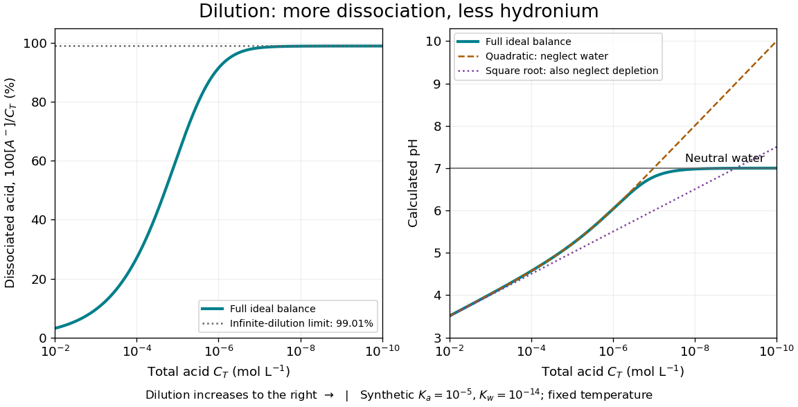
Dilution increases the weak acid dissociation fraction while raising pH in a synthetic aqueous chemical equilibrium
. Details. 
The diagram uses stipulated dimensionless acid dissociation constant and self-ionization of water ion product at fixed temperature; these are model inputs, not measurements of a named substance. It solves the weak acid mass and charge balances. At , the calculated weak acid dissociation fraction is about and pH about ; at , they are about and . More acid units are dissociated as a fraction of the total, yet fewer hydronium ions occur per volume.
At extreme dilution, self-ionization of water makes approach , so pH approaches for the chosen model. The limiting weak acid dissociation fraction is , rather than exactly one. The calculation assumes pure added water, a neutral monoprotic acid, and no competing chemical reactions; actual contamination becomes increasingly important as falls.
A monoprotic acid supplies one proton per acid unit in the acid-base chemistry model under consideration. Acetic acid is an example. Several successive proton transfers require several acid dissociation constants and a larger set of chemical species.
For real , deformation into the upper half-plane separates a logarithmically singular endpoint at zero from the smooth endpoint at one. The first contributes the exact logarithmic term displayed. The second yields its factorial asymptotic expansion by Watson's lemma. The two endpoints must both be retained; repeated integration by parts without treating the logarithmic singularity loses its leading contribution.
A cut-off endpoint integral with amplitude has a logarithmic rather than a Taylor endpoint expansion. Set and expand against . The derivatives of the gamma function at one supply the logarithmic moments: and . Other peaks or singularities must be treated separately before applying this endpoint result to a whole integral.
For with positive and , differentiation cancels the logarithmic denominator and gives . Integrating this derivative expresses as a finite parameter-Laplace integral plus . The elementary lower bound gives the displayed remainder, smaller than every logarithmic term at fixed . Watson's lemma then determines all coefficients from the finite integral's endpoint Taylor series.
Use circulation to summarize how much a velocity field runs along an oriented closed curve , such as a circle around a fluid vortex. Its definition is the line integralwhere is tangent to in the chosen direction. Reversing that direction reverses the sign of circulation. Its units are , because velocity is multiplied by a length. Counterclockwise circulation in the horizontal plane is positive when the chosen unit normal vector is , according to the right-hand rule.
For solid-body rotation , a counterclockwise circle of radius has constant tangential velocity . Multiplying by its circumference givesFor the potential line vortex , the same circle instead gives , independent of . Stipulate , and : both velocity fields have , although their vorticities in the fluid are and zero respectively. On a circle of radius , their circulations are and . The comparison plot in vorticity shows this difference in radius dependence.
The bridge between circulation and vorticity is Stokes theorem:Here the velocity field must be continuously differentiable on a neighborhood of the entire spanning surface inside the fluid, and its boundary orientation must match the unit normal vector . For solid-body rotation, the disk is admissible and its surface integral is . For the potential line vortex, the origin is singular and excluded from the fluid: a disk crossing it is not admissible. On an annulus, Stokes theorem instead gives , with both circulations here measured counterclockwise; the induced inner boundary direction is clockwise. Nonzero circulation therefore does not imply nonzero local curl in the available fluid. [ref]
https://davidtong.org/pdfs/teaching/fluid-mechanics/fluids1.pdf. David Tong, Fluid Mechanics, section 2.2, circular-flow example
This is useful because Stokes theorem lets a local vorticity measurement determine a loop's circulation when a suitable surface exists, while Kelvin's circulation theorem tracks circulation along a moving material curve. The beauty is the precise link between a local derivative and a global line integral, with the domain deciding which conclusions are valid.
Kinetic helicity measures the alignment and linking of a velocity field and its vorticity. It is the volume integral of , with boundary conditions needed for its conservation.
Enstrophy measures squared vorticity: a local density is , and its spatial integral or ensemble mean gives a global measure. In homogeneous incompressible flow, viscous dissipation satisfies . Vortex stretching can produce enstrophy in three dimensions; kinematic viscosity destroys it.
A vortex tube is a bundle of vortex lines bounded by a surface to which vorticity is tangent. Circulation measures its vorticity flux. Stretching a nearly incompressible tube reduces its cross-sectional area and increases its vorticity. The Burgers vortex is a local model in which this concentration balances viscous diffusion.
Hydrodynamic impulse per unit density is for localized vorticity. In unforced all-space incompressible flow its derivative vanishes when far-field fluxes vanish. For a spherical all-space limit, ; a dipolar velocity tail makes the distinction from a bare momentum integral important.
In an unbounded incompressible fluid with localized vorticity and no added harmonic background, velocity is reconstructed by . Its multipole expansion relates hydrodynamic impulse to a dipolar far-field velocity.
There are unlisted articles, also show them or only show them.