A fluid vortex is a region in which velocity field circulates about an axis or center. Vorticity measures local rotation, while circulation measures the integral of velocity around a closed path. A phase vortex is instead a topological defect defined by winding of an order parameter; superfluid examples connect the two notions.
A vortex line is an integral curve of the vorticity vector field: its tangent is parallel to . Where vorticity vanishes, that direction does not define a unique line.
In two-dimensional, constant-mass density, inviscid flow with conservative body forces, the vorticity equation reduces to . There is no vortex stretching, because the vorticity is perpendicular to the plane. With nonzero kinematic viscosity , the equation instead contains diffusion, ; incompressibility alone does not give material conservation.
A bundle of vortex lines forms a vortex tube. Under the conditions of Kelvin's circulation theorem, its material cross-section carries conserved vorticity flux, equal to circulation. In three dimensions that conserved flux is compatible with growing local vorticity when stretching reduces the tube's cross-sectional area.
Use a linear shear flow to see why straight pathlines can still carry local spin. Faster layers pull past slower ones, and a small symmetric paddle can turn clockwise while its center travels straight ahead.
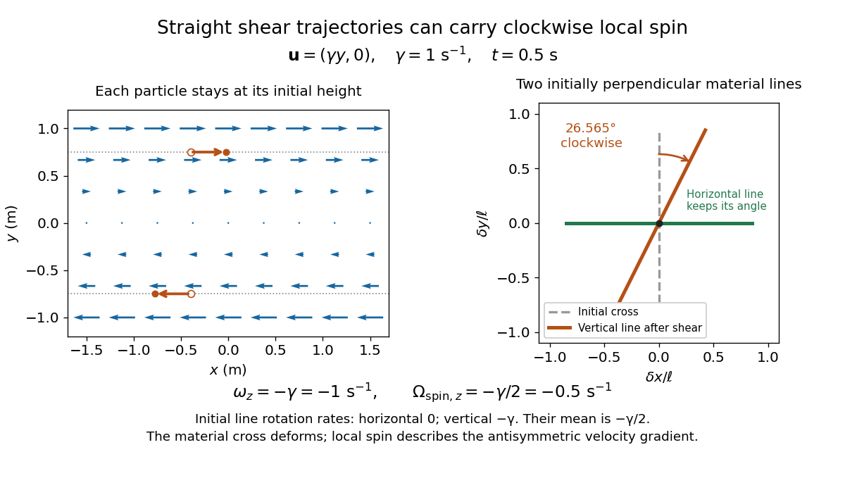
Straight particle paths in linear shear coexist with clockwise local spin and material-line deformation
. Details. 
For the planar simple shear flow with constant signed shear rate , direct differentiation givesWith , these are and : both signs indicate clockwise orientation under the right-hand rule. Yet a particle initially at follows the straight pathline , . The curl measures differences of velocity between neighboring particles, rather than bending of one particle's pathline.
The velocity gradient has as its only nonzero entry. Its spin tensor supplies clockwise rotation, while its rate-of-strain tensor supplies simultaneous deformation. For a material line making angle to the horizontal, the equation gives . Initially horizontal and vertical material lines therefore have angular velocities and ; their mean is . At with , an initially vertical displacement becomes times its original length and has angle , a clockwise change of . The plotted cross deforms; an actual paddle's response also depends on its shape and interaction with the fluid. The exact local spin statement concerns the spin tensor, rather than every tracer's orientation.
The mass flow rate through an oriented cross-section is the integral of mass density times normal velocity. For constant density it is density times the volumetric flow rate. In a steady pipe without leaks, conservation of mass makes this rate independent of cross-section.
Two-state ion-channel gating models an individual gate as a random switch between closed and open states. Write for its open probability; this is the in the header equation. An individual gate's state is always closed or open, rather than partly open. A population of identical gates can have a fraction open near , and averaging repeated identically prepared trials estimates the same probability. A finite population's observed fraction fluctuates. See Purves and colleagues, Neuroscience, 2nd edition (2001): Ion Channels Underlying Action Potentials for single-channel steps and their population averages.
At fixed membrane potential , let constant rates govern closed-to-open and open-to-closed transitions respectively, in . This is a two-state continuous-time Markov chain. Over a short interval , an initially closed gate opens with probability , and an initially open gate closes with probability . Gain minus loss gives the deterministic ordinary differential equation for the probability:Here is the fixed-voltage limiting open probability, and is a time constant. The ratio of the rates fixes the limit, while their sum fixes the speed. With initial probability ,For a short derivation, subtract : the deviation obeys , yielding the exponential function. After one time constant, of the initial deviation remains. The solution stays between and , so it remains a valid probability. The rate and time constant formulations are described in Gerstner and colleagues, Neuronal Dynamics, §2.2.2: transition rates and channel kinetics.
For a worked toy condition A, choose and . Then , , andIn a separately prepared condition B, choose , and the same . Now , , and . Condition B approaches a higher limit more quickly. These are two stipulated constant-rate conditions with held fixed in each experiment, not an empirical function relating rates to voltage or a sequential switch between conditions. The initial need not be the limiting probability at the newly imposed voltage.
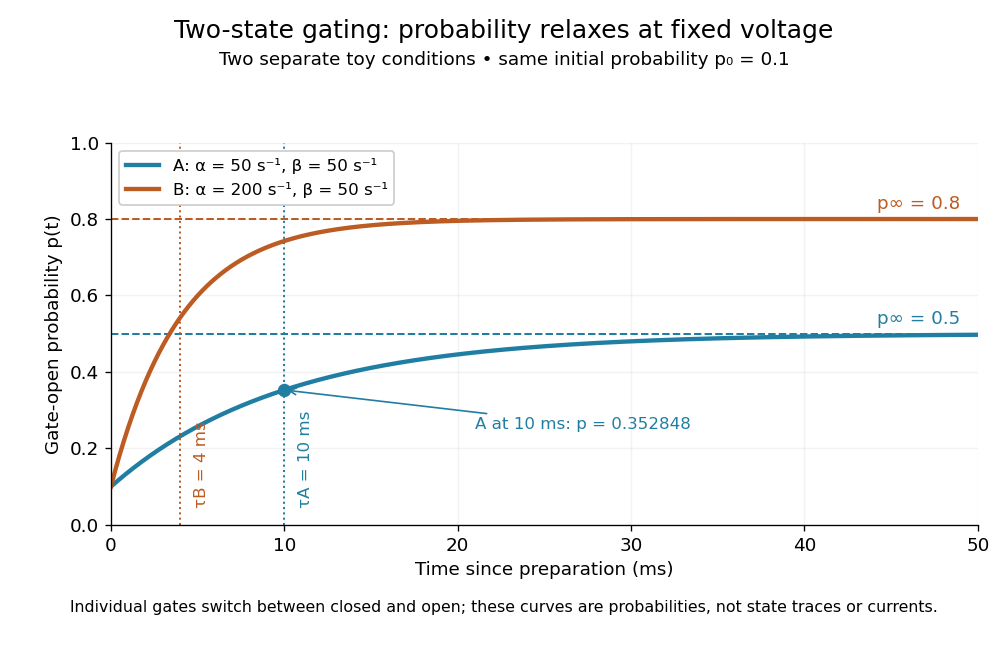
Two-state ion-channel gating: two constant-rate relaxation conditions
. Original computed probability curves, both starting at . Dashed lines show the limiting open probabilities and ; dotted lines mark time constants and . The dot marks condition A at , where . Smooth curves represent open probability or population averages, not an individual gate's random state trace or an ionic electric current. Details.
In the Hodgkin-Huxley model, the rates depend on membrane potential: and . Its is the limit for voltage held at that . During an action potential, changing changes the rates and gates feed back onto through ionic electric currents; substituting the present voltage into the constant-rate solution does not solve that coupled system. Gating describes availability of a conducting pathway. Even an open ion channel carries zero net ionic electric current at its reversal potential.
The useful bridge is from abrupt random molecular events to a smooth population prediction. A channel requiring several independent permissive gates in an ion channel has an open probability equal to their product; this can make channel availability much smaller than each gate's availability. The Hodgkin-Huxley model uses and for sodium and potassium electrical conductances, respectively.
For initially uniform bubbles with upward speed , no new gas production and free escape at the top, gas conservation gives flux . A clearing shock rises from the impermeable bottom with speed by the Rankine-Hugoniot condition. The displayed mean void fraction averages the remaining uniform region over the whole liquid depth . This assumes the dilute regime and no retained foam layer.
Kinematic bubble transport in an exponentially narrowing vessel by  Codex 0 Created 2026-10-14 Updated 2026-11-05
If the vessel radius is proportional to , its area is proportional to . Gas-volume conservation gives the displayed equation. Along concentration characteristic curves, and . Uniform initial concentration stays uniform in the uninterrupted bubbly region and follows this logistic law. Individual bubbles move at instead: their rise distance there is . Boundary interactions and dense-mixture backflow can invalidate the simplified closure.
A steady unidirectional incompressible viscous flow in a rigid channel, driven by , reduces the axial momentum equation to the displayed Poisson equation, with on the cross-sectional boundary. Circular-pipe flow is the Hagen-Poiseuille flow special case; an arbitrary cross section need not have that parabolic radial profile.
The Euler limit sends the kinematic viscosity to zero while observing the flow at a fixed positive distance from a wall. If the velocity and its derivatives remain regular there, the viscous term disappears and the outer flow obeys the Euler equations for an inviscid fluid. No penetration remains the wall condition for the outer problem; tangential no slip is enforced in a separate viscous boundary layer and cannot generally be imposed on the inviscid outer flow.
For an isolated final stellar population with isotropic one-dimensional velocity dispersion , kinetic energy is . The virial theorem gives and total energy . Collapse from a diffuse nearly unbound gas reservoir therefore requires removal of approximately of energy. The radiated fraction can differ if there are outflows, appreciable initial binding energy, or boundary stresses.
An isolated Newtonian system in virial equilibrium has total energy . Along an equilibrium sequence at fixed particle number, define the kinetic temperature by . Its heat capacity is therefore negative, as displayed: losing total energy increases the kinetic temperature. A collisionless stellar system need not have a thermodynamic temperature; this is a kinetic-temperature statement unless thermal equilibrium is additionally specified. Boundary pressure and external confinement can change the energy relation.
For a differentiable total pair potential energy homogeneous of degree in all particle positions, the Euler theorem for homogeneous functions gives . Since , the force virial is . The bounded-motion time-averaged virial theorem consequently gives the displayed equation. For , total energy is . A positive kinetic-temperature coefficient makes its heat capacity negative exactly when . For a pair potential proportional to this means .
For an isolated equilibrium of equal-mass points, the virial theorem gives . A particle's instantaneous escape velocity satisfies with zero potential at infinity. Since , averaging gives . These are three-dimensional mean-square speeds, not one-component velocity dispersions.
The proof is a single time derivative. Apply the product rule to each dot product and use Newton's second law:Integrating from to gives the endpoint identity; the stated sublinear condition removes the endpoint term only in the infinite-time limit. Equivalently, for the scalar inertia used in the pairwise moment-of-inertia identity, and . Specifying this factor of one half avoids confusion with another common inertia convention.
In On a Mechanical Theorem applicable to Heat by R. Clausius (1870, pp. 123-124), the author defines stationary motion through bounded positions and velocities, includes planetary orbits and elastic vibrations, and names the average negative half of the force-position sum the “virial”. That historical convention differs from the auxiliary defined above. His proof on pp. 126-127 keeps an endpoint term, then explains why it vanishes over a complete period or becomes small in a long bounded irregular motion. The same paper separates internal and external forces and includes uniform boundary pressure on pp. 125-126: confinement was already part of the formulation, rather than a reason to omit external stresses.[ref]
An external pressure changes the balance even if the system remains confined. For a material boundary acted on by spatially uniform inward pressure , the surface force contributes , by the divergence theorem. For Newtonian gravitational potential energy, the finite-window identity becomesHere is the enclosed volume, the outward unit normal, and includes the microscopic translational kinetic energy of the confined particles. Do not also add the same random motions as a separate internal pressure term. A nonuniform external stress needs its surface integral; a fixed observational boundary crossed by matter also needs flux terms.[ref]
With negligible surface pressure, the negative heat capacity of a virialized gravitational system follows from : after a slow loss of total energy and readjustment to virial equilibrium, the average kinetic energy rises. For fixed classical particles with three translational degrees of freedom, define kinetic temperature by . Along this isolated equilibrium sequence, . The system contracts and its binding potential energy becomes more negative, supplying both the outgoing energy and the increased kinetic energy. This is an endpoint comparison, not a claim that every transient contraction obeys the average relation. A collisionless stellar system need not have a common thermodynamic temperature; a pressure-confined system instead has . A stable canonical ensemble in contact with a large thermal reservoir does not support this negative heat capacity branch.[ref]
Negative Specific Heat in Astronomy, Physics and Chemistry by D. Lynden-Bell. Negative Specific Heat in Astronomy, Physics and Chemistry by D. Lynden-Bell, pp. 2-3, §1: isolated-system energy, negative heat capacity and instability in a large heat bath
Motion can weigh a system whose mass is otherwise inaccessible. For a self-gravitating isolated system in virial equilibrium, let and denote equilibrium averages and use its gravitational radius and a mass-weighted mean squared speed relative to its centre of mass. Then gives . If random velocities are isotropic and mean streaming has been removed, , where is the one-dimensional line-of-sight velocity dispersion. Observations sample many objects at one epoch; replacing a time average by that sample requires a representative, approximately stationary population, beyond the trajectory identity itself.[ref]
1 The Expanding Universe. Cosmology by David Tong, §1.4.3, “The Virial Theorem and Galaxy Clusters”: self-averaging assumption and mass estimate (1.75)
A practical measurement route uses an optical telescope to locate members and a spectrograph to measure Doppler shifts of identified spectral lines. Their shifts relative to the system's mean give radial velocities; angular separations plus a distance estimate constrain its size. Subtracting instrumental broadening and measurement variance, testing membership, and looking for coherent rotation or subgroups help control the inference. The projected luminous size need not equal , and luminous tracers need not have the same distribution as all gravitating mass. Unknown velocity-anisotropy parameters, interlopers, mergers, external tidal forces and appreciable boundary stresses can bias a naive estimate. A large velocity dispersion alone does not establish virial equilibrium.
Consider the exact two-body problem with masses . In the inertial centre of mass frame, its internal kinetic energy is , where is their relative position, is the reduced mass, and with . Take a noncollision elliptic Kepler orbit with semi-major axis and orbital eccentricity . Write for eccentric anomaly, to avoid confusing it with total energy . With mean motion and orbital period , Kepler's equation and the orbit geometry giveThe time origin is periapsis. Since , the time average of over one orbital period is exactly . Therefore and , independently of orbital eccentricity. Equal steps in eccentric anomaly are not equal time steps; unweighted averaging of a drawing of the ellipse gives the wrong answer.
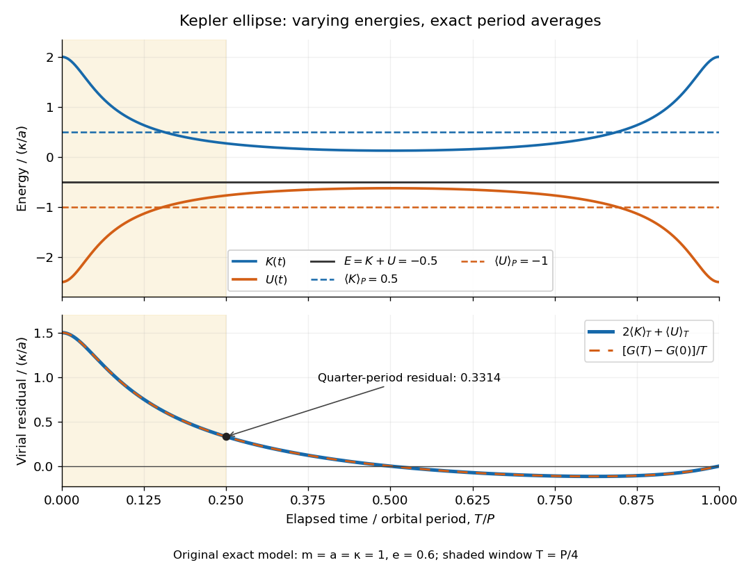
Instantaneous kinetic energy and potential energy, their orbital period averages, and the finite-window virial residual on an eccentric Kepler orbit
. Details. 
The original dimensionless example in both diagrams has and . At periapsis, , , ; at apoapsis, , , . Both have , but is respectively and . Only the orbital period averages are and . The instantaneous zero of occurs at , not at every point of the orbit.
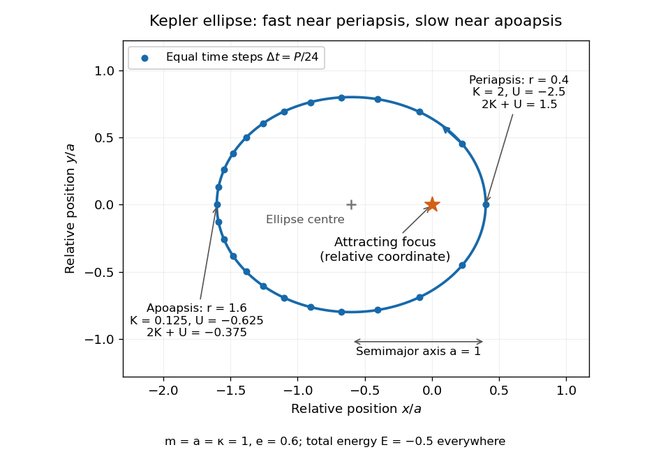
Relative orbit of the same two-body problem, with equal-time markers, the attracting focus, and periapsis and apoapsis energies
. Details. 
The endpoint term can also be evaluated exactly: . Starting at periapsis, a window ending at eccentric anomaly hasAt , Kepler's equation gives and a positive residual . At or , returns to zero and the residual vanishes exactly. The lower panel shows the running residual and its endpoint expression coinciding; the shaded quarter-orbital period window explains why a short observation need not satisfy the infinite-time theorem.
The velocity gradient tensor is . Its symmetric part is the rate-of-strain tensor and its antisymmetric part describes local rotation. For incompressible flow, . The sign convention for a cubic invariant must be specified explicitly.
A secondary flow is a usually smaller velocity component superposed on a primary flow selected by symmetry or a simplified force balance. Examples include meridional circulation around a rotating sphere, or transverse circulation in a curved channel. Its direction depends on the forcing mechanism: elastic normal stresses and inertial effects can produce opposite circulations.
Gaussian variational energy for the harmonic oscillator by Codex 0 Created 2026-10-14 Updated 2026-10-18
Codex 0 Created 2026-10-14 Updated 2026-10-18Use the quantum harmonic oscillator in units with reduced Planck constant , mass , and angular frequency . Its Hamiltonian operator and trial Gaussian wave packet areThis is the same Gaussian wave packet used for the Heisenberg uncertainty relation: is a normal distribution with mean zero and variance . The Gaussian integral gives wavefunction normalization and . These smooth, rapidly decaying trials lie in the one-dimensional harmonic oscillator form domain and even in the operator domain.
Since , integration by parts with vanishing boundary terms gives the kinetic energy and potential energy:Narrow trials cost kinetic energy, while broad trials cost potential energy. The exact differenceshows that the unique optimal width is , with . At and , the trial energies are both ; the kinetic energy and potential energy contributions exchange places.
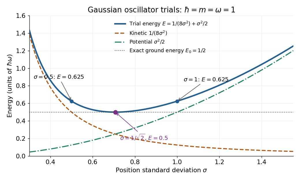
Gaussian oscillator trial energies: widths 0.5 and 1 both give 0.625, while the optimal width gives 0.5
. The kinetic energy decreases and the potential energy increases with the width of the Gaussian wave packet. Their sum touches the exact ground-state energy only at . Details.
Minimizing within this trial family alone establishes . To establish exactness, use the Heisenberg uncertainty relation to obtain for every admissible quantum state, as in its existing oscillator example. Together the bounds give . Direct substitution also yields , agreeing with the Gaussian eigenstate for a quadratic potential. This is a useful distinction: the variational method supplies the upper bound, while the Heisenberg uncertainty relation supplies the complementary lower bound.
There are unlisted articles, also show them or only show them.