
The protein primary structure specifies the ordered amino acid residues of each polypeptide chain, joined through peptide bonds. A chain is conventionally written from its N-terminus to its C-terminus. In the broader chemical sense, a complete protein primary structure also specifies covalent bond crosslinks between chain positions, including protein disulfide bonds; a bare sequence string leaves that information unstated. This describes chemical connectivity rather than the spatial arrangement of protein tertiary structure or protein quaternary structure. See IUPAC Gold Book: primary structure, sequence and chain crosslinking and IUPAC-IUB, 3AA-16: writing residue sequences from the amino end. Some conventions reserve protein primary structure for sequence alone and call the complete chemical connectivity the covalent structure; the distinction should be stated when comparing descriptions. See IUPAC-IUB polypeptide-conformation recommendations, section 6.1: the narrower sequence-only convention.
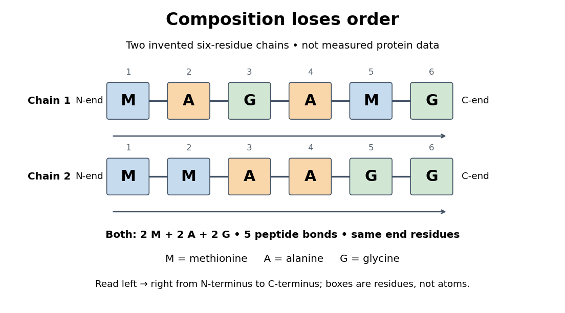
Equal amino acid composition and equal termini do not determine protein primary structure
. Original toy polypeptide chains MAGAMG and MMAAGG, read from the N-terminus to the C-terminus. Each contains two methionine, two alanine and two glycine amino acid residues, but their internal order differs. Letters denote chain positions rather than free amino acids; lines denote peptide bonds. Neither string is identified as a natural protein or a measured sequence. Details.In this toy example M denotes methionine, A alanine and G glycine. Both polypeptide chains have six amino acid residues, five peptide bonds, an M at the N-terminus and a G at the C-terminus. Their amino acid composition is identical, yet position 2 is A in MAGAMG and M in MMAAGG. There are distinct orders with these counts, a multinomial coefficient. Even fixing those two end residues leaves orders. The counts constrain the answer without determining it.
For multiple polypeptide chains, record each sequence separately and specify any protein disulfide bonds between cysteine positions. Mature insulin, for example, has an A chain of 21 amino acid residues and a B chain of 30 amino acid residues. Their combined 51 residues give peptide bonds, rather than the 50 of one unbroken 51-residue chain. See Cooper, The Cell: insulin's two chains and cysteine crosslinks, figure 2.16. A protein disulfide bond joins side groups; it does not concatenate the C-terminus of one chain with the N-terminus of another. The three insulin protein disulfide bonds connect A6 to A11 within the A chain, and A7 to B7 and A20 to B19 between chains. Positions are numbered from each chain's N-terminus. See Replacement of the interchain disulfide bridge-forming amino acids A7 and B7 by glutamate impairs the structure and activity of insulin: native disulfide positions.
Why keep this information? Protein primary structure lets us distinguish changes of chemical identity from changes of shape, and compare corresponding positions between proteins. Protein folding can bring distant amino acid residues together at a protein binding site while preserving their sequence. The attractive idea is that a readable linear record can constrain a complicated three-dimensional object; it is not, by itself, a guarantee of a unique fold in every environment. See protein folding and the ribonuclease A refolding experiment. Merely bending an intact chain preserves its protein primary structure; hydrolysis of a peptide bond, or changing which positions a protein disulfide bond connects, changes its chemical connectivity.
A protein domain is a distinguishable structural and functional region of a protein. A catalytic protein domain and a binding protein domain can carry out different tasks within one chain.
A protein tyrosine phosphatase acts on phosphotyrosine residues. Removal can undo a particular receptor modification; its consequences for the whole signal transduction pathway depend on the target.
Autophosphorylation is phosphorylation of a protein kinase by its own catalytic activity or that of another member of the same protein kinase assembly. Distinguish modification within one chain from trans-autophosphorylation between partners.
A molecular chaperone is a protein that assists other proteins in reaching or maintaining useful arrangements, for example by limiting unwanted association during protein folding. Assistance does not rewrite the client's protein primary structure. In a crowded cytoplasm, reducing protein aggregation can make successful protein folding more reliable. See Cooper: molecular chaperones and folding assistance.
Archaea are a major evolutionary lineage distinct from bacteria. The cellular comparison here concerns the prokaryotic members of archaea; see two-domain system for broader clade usage. Their biological cells have a nucleoid rather than a membrane-bounded cell nucleus, yet aspects of DNA replication, transcription and biological translation resemble those of eukaryotes. Their characteristic lipids differ chemically from the usual bacterial membrane lipids, and their cell walls, when present, lack peptidoglycan. See OpenStax Biology 2e, 22.2: archaeal distinctions.
Some archaea perform methanogenesis, producing methane as part of their metabolism. Archaea also inhabit ordinary soils and oceans: extreme habitats do not define the lineage. See OpenStax Biology 2e, 22.1: moderate and extreme environments. Woese and Fox's 1977 analysis of ribosomal RNA distinguished the methanogenic group they called archaebacteria from typical bacteria. Their proposed three primary lines of descent were a historical interpretation, rather than the final resolution of deep phylogenetics. See Woese and Fox, 1977: Phylogenetic structure of the prokaryotic domain.
Bacteria are a major evolutionary lineage of organisms with prokaryotic cellular organization. Escherichia coli and cyanobacteria illustrate its variety: the same broad cellular plan supports different kinds of metabolism. Most bacteria have a cell wall containing peptidoglycan; archaea do not have peptidoglycan walls. A cell wall and a cell membrane are distinct structures, and some bacteria lack a cell wall. See OpenStax Biology 2e, 22.2: bacterial envelopes.
The usefulness of recognizing bacteria extends beyond naming: it identifies a shared evolutionary background for comparing genes, proteins and cellular mechanisms. A familiar shape or the absence of a cell nucleus alone cannot distinguish bacteria from archaea; molecular comparisons, including ribosomal RNA, supply additional evidence.
A program action that associates a value with a target name. For Python
x=2+3*4, evaluate the right-hand program expression and bind x to its result. [ref]https://docs.python.org/3.14/reference/simple_stmts.html#assignment-statements. Python language reference, section 7.2: assignment to an identifier and evaluation of the right-hand side
A program construct that is evaluated to obtain a value, potentially with side effects or failure. An arithmetic mathematical expression is one example; its abstract syntax tree records how operands and operations nest.
A name used by a program, such as
x in a variable assignment. An abstract syntax tree can record the name without determining which value it denotes.A parser recognizes how text fits a programming language syntax and can construct a parse tree or abstract syntax tree.
Recognition of lexical tokens in program text before or during parsing.
A processor register identifying the current position in a stack, commonly a call stack; the exact convention depends on the architecture. Restoring a stack pointer selects the saved stack position, rather than copying the whole call stack.
A context switch transfers CPU execution from one operating-system process or software thread to another while preserving enough execution context for the suspended task to resume. The operating-system kernel saves the outgoing task's processor registers, including its resume program counter and stack pointer, and restores the incoming task's saved state. Hardware entry and software switching divide this work differently across architectures; the diagram groups them into logical save and load steps. During the transition the same CPU executes the operating-system kernel's scheduler and switching code. [ref]
https://pages.cs.wisc.edu/~remzi/OSTEP/cpu-mechanisms.pdf. Remzi H. Arpaci-Dusseau and Andrea C. Arpaci-Dusseau, Operating Systems: Three Easy Pieces, chapter 6, section 6.3: saving and restoring context
For a schematic switch from A to B, let A's resume program counter be , its stack pointer , and one illustrative data processor register contain 7. B's saved values are . Saving A retains in A's execution context; loading B establishes before B resumes. These are selected fields, not a complete architecture-specific execution context. Later restoring A recovers its 7 even though B has used the same physical processor register for 42.
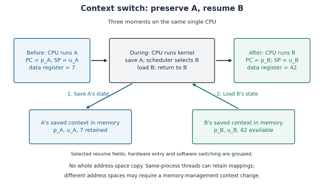


The useful invariant is that each suspended task retains its own resume state, so another task's use of the processor registers does not erase it. This is what makes repeated turns under round-robin scheduling possible. Saving an execution context does not copy the entire address space. Switching between software threads of one operating-system process can retain the same address space; switching between operating-system processes with different address spaces may also require changing the memory management unit's translation context, such as the active page table and associated address space identifier, depending on the architecture. Their contents remain in computer memory. [ref]
https://pages.cs.wisc.edu/~remzi/OSTEP/threads-intro.pdf. Remzi H. Arpaci-Dusseau and Andrea C. Arpaci-Dusseau, Operating Systems: Three Easy Pieces, chapter 26, introduction: thread contexts and shared address spaces
Entering the operating-system kernel through an interrupt, synchronous processor exception or system call does not automatically imply a context switch to another task. The handler may return to the same task; process scheduling determines whether another runnable task should take over. A context switch consumes time, and a changed memory cache or translation lookaside buffer working environment can add subsequent costs. Those costs are excluded from the toy process scheduling timelines, which are calculations rather than operating system benchmarks. [ref]
https://pages.cs.wisc.edu/~remzi/OSTEP/cpu-mechanisms.pdf. Arpaci-Dusseau and Arpaci-Dusseau, OSTEP chapter 6, section 6.3: continue the current process or switch
[ref]https://pages.cs.wisc.edu/~remzi/OSTEP/cpu-sched.pdf. Arpaci-Dusseau and Arpaci-Dusseau, OSTEP chapter 7, section 7.7: direct and indirect switching costs
The total duration a task spends runnable but waiting for a CPU, including later waits after scheduling preemption. Under the zero-overhead, no-input-output-blocking assumptions of process scheduling, elapsed time partitions into useful execution and such waiting, so , where is scheduling turnaround time and is the total CPU burst. Thus C under round-robin scheduling has . If a task also spends time blocked on input-output, that blocked duration belongs to scheduling turnaround time but must not be counted as scheduling waiting time.
// Target: computer-science.bigb
The duration from a task's arrival until its completion : . It includes execution and all intervening waits. For A under round-robin scheduling in process scheduling, , despite a scheduling response time of zero.
The delay from a task's arrival until its first execution : . This measures access to initial CPU service, rather than completion of an entire user request. For C under round-robin scheduling in process scheduling, ; its scheduling turnaround time is instead .
Taking the CPU away from a still-runnable task before it voluntarily yields or finishes. Round-robin scheduling uses scheduling preemption when a scheduling quantum expires, commonly using a timer interrupt to regain control. Kernel preemption is the more specific question of whether an execution already within the operating-system kernel can be suspended for another runnable context.
Serve the front of a FIFO queue of runnable tasks for at most one scheduling quantum. If the task finishes or must wait for input-output, it leaves the CPU earlier; if it remains runnable after consuming its allowance, append it to the rear of the ready queue. In the example under process scheduling, the ready queue at time 2 is B, C, A: B arrived at time 1, C joins at the boundary, then A is requeued. That one convention determines the subsequent order.
There are unlisted articles, also show them or only show them.