
An intracellular receptor recognizes a ligand inside a biological cell, including in the cytoplasm or cell nucleus. Some intracellular receptors regulate transcription after binding a membrane-permeable signal; an intracellular receptor does not universally imply direct control of DNA. See the receptor-location reference under receptor.
A cell-surface receptor detects an extracellular signal at the cell membrane. Its changed state affects the intracellular side, coupling reception to signal transduction or directly to an ion channel's opening.
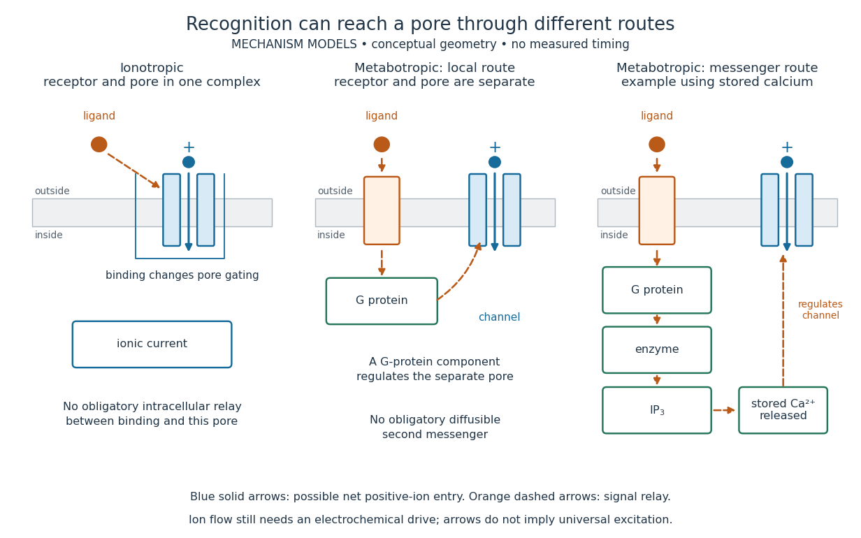
A metabotropic receptor couples ligand recognition to intracellular signal transduction, which can regulate a separate ion channel, alter enzyme activity or change gene expression. In the usual neurotransmitter context, metabotropic receptors are G protein-coupled receptors: receptor activation is relayed by a G protein. There need not be a change in membrane potential at all. [ref]
Two routes should be distinguished. An activated G protein can regulate an ion channel locally at the cell membrane, without an obligatory diffusible second messenger. Alternatively, it can regulate an enzyme that changes the availability of a second messenger, such as cAMP or inositol trisphosphate. Downstream proteins then change channel opening, phosphorylation or other cellular activities. The receptor, G protein, second messenger and final target are distinct components; an activated G protein is a relay protein, rather than itself a small-molecule second messenger.[ref]
General Principles of Cell Communication. Figure 15-15
Do not turn this useful chemical synapse classification into the claim that every receptor is a GPCR, or that every indirect response must pass through a G protein. For example, the insulin receptor is an enzyme-linked cell-surface receptor whose intracellular catalytic activity initiates protein phosphorylation. Intracellular receptors supply another category. “Metabotropic” commonly names the GPCR branch in neuroscience; the broader idea of biochemical coupling does not make all non-channel receptors structurally identical. [ref]
Separating recognition from execution allows signal amplification and branching. A persistently activated receptor can activate several relay proteins; a regulated enzyme can produce many second messenger molecules. As an explicitly invented count example, suppose one activated receptor activates four relay proteins during one interval, and each relay activates a distinct enzyme that produces fifteen second messenger molecules during the next interval. With sufficient substrates and no loss, this gives molecules. Those counts do not specify a physiological gain or response duration. A directly gated ion channel also passes many ions while open, so amplification is not an exclusive property of metabotropic receptors: always name the input and output being compared. [ref]
A particularly instructive electrophysiology experiment separated a chemical trigger from the ion channel carrying its eventual electric current. In 1987, Hirono, Ito and Sugiyama injected messenger RNA from rat brain into frog egg cells, then tested acquired responses to neurotensin and muscarinic acetylcholine stimulation. Under voltage clamp at , neurotensin elicited transient, oscillatory inward electric currents after a delay of several tens of seconds. This delay refers to that response and preparation. Reversal potential measurements implicated increased permeability to chloride anions, rather than a pore specific to the applied ligand. Both neurotensin and acetylcholine responses were inhibited by pertussis toxin, which interferes with susceptible G proteins, and by intracellular EGTA, which binds free calcium. Injecting inositol trisphosphate mimicked the responses; a large prior dose of inositol trisphosphate reduced subsequent responses to either extracellular signal. These interventions implicate a shared intracellular relay and calcium-dependent channel opening.[ref]
The informative comparison with the nicotinic acetylcholine receptor experiment is mechanistic: an extracellular ligand can produce an inward electric current either by directly gating the pore or by mobilizing an intracellular second messenger and stored calcium that activate another pore. Intracellular inositol trisphosphate bypasses reception, whereas EGTA tests the need for free calcium. However, neither inhibition nor mimicry alone identifies every molecular connection: a perturbation can affect several targets, and an injected mediator can activate a pathway without proving that it is the only natural route. The egg cell's endogenous machinery and the mixed messenger RNA preparation also limit extrapolation to an intact neuron. The experiment establishes functional coupling in its preparation, rather than the exact molecular composition or timing of every metabotropic receptor.
Even G protein-dependent channel regulation need not involve a lengthy second messenger cascade. Pfaffinger and colleagues reported in 1985 that acetylcholine-evoked potassium channel activation in embryonic chick atrial cells required intracellular GTP, a guanine-containing nucleotide, and was abolished by pertussis-toxin pretreatment. Changes in cyclic nucleotides, including cAMP, did not account for the channel response. The report discusses intrinsic activation delays of roughly –, illustrating relatively rapid metabotropic receptor action. These observations support a G protein coupling step without cyclic-nucleotide second messengers; they do not by themselves exclude every possible intermediary or prove the specific subunit-channel interaction.[ref]
A small timing model makes the extra steps visible without inventing an experimental trace. Let jump from zero to one at and remain on. For a direct-gating model output , one relay variable , and its downstream output , take zero initial conditions andAll outputs are normalized dimensionless variables; they are neither recorded electric currents nor fitted concentrations. With illustrative time constants , and , their exponential function solutions for areInitially , while because its relay must first build up. Both outputs eventually approach one. Equal normalized final values do not imply equal biological amplitudes or absence of signal amplification; normalization deliberately removes that question.
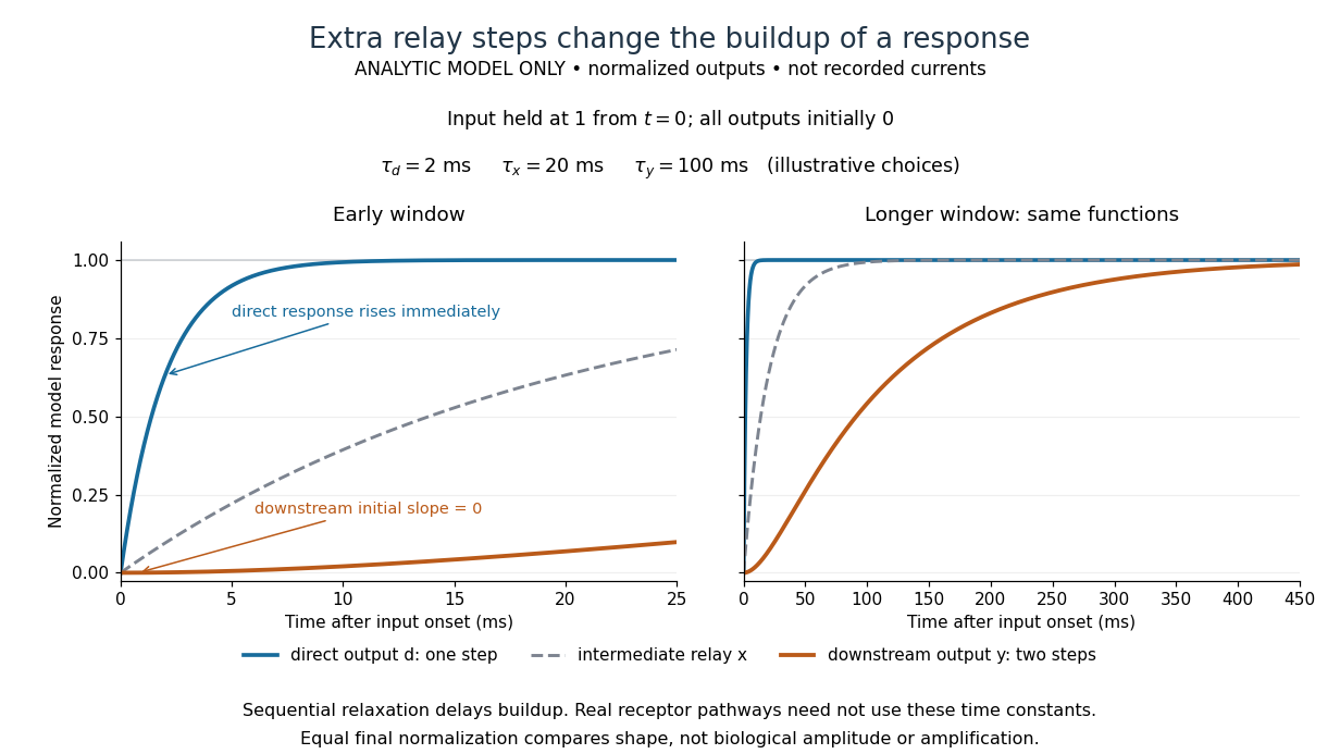
The model's useful feature is the delayed buildup created by sequential relaxation, not its arbitrary numbers. Actual kinetics also depend on ligand delivery, relay deactivation, neurotransmitter clearance and the final target. A local G protein route can act promptly, while an ionotropic receptor can remain active during continued exposure or feed a longer-lasting intracellular response. The beauty of metabotropic receptor coupling is its flexibility: the same recognition event can adjust electrical responsiveness and other cellular tasks through different targets. To classify an observed response, combine timing with molecular identity and controlled perturbations.
An ionotropic receptor is a receptor in which binding of a ligand directly gates an ion channel within the same protein complex. The binding site detects the chemical signal; the pore supplies a path across the cell membrane. At a chemical synapse, a neurotransmitter therefore changes synaptic conductance without an obligatory intervening G protein or second messenger. [ref]
A familiar example is the nicotinic acetylcholine receptor of skeletal muscle: acetylcholine binding opens a pore passing cations, including sodium and potassium. The muscarinic acetylcholine receptor instead uses intracellular signal transduction; the same neurotransmitter can engage different mechanisms. Direct gating does not mean that an ionotropic receptor pumps ions: electrochemical gradients drive passage through the open ion channel. Nor does “ionotropic” specify excitation. The reversal potential, initial membrane potential and other conductances determine whether the effect favors an action potential, causes hyperpolarization, or supplies shunting inhibition. [ref]
A concrete electrical approximation separates opening from drive. Let identical ion channels each have open-channel electrical conductance and opening probability . At fixed membrane potential , with common reversal potential , the expected value of inward-positive electric current isFor stipulated values , , , and , the mean open count is , the population electrical conductance is and . One open ion channel carries . These are illustrative values, not measurements. At , the net electric current vanishes despite open ion channels; neither binding nor opening alone determines the readout. The approximation omits changes in ion concentrations and voltage-dependent open-channel electrical conductance.
A motivating experiment made the elementary electrical events visible. As Bert Sakmann recounts, chronically denervated frog muscle fibers had acetylcholine-sensitive receptors spread beyond the original nerve contact. Mild enzyme treatment exposed the cell membrane; a polished glass pipette sealed over a small patch to reduce background noise. Two intracellular electrodes held the local membrane potential through voltage clamp, while the patch pipette recorded tiny electric currents. Applying suberyldicholine, a ligand that activates the acetylcholine receptor and prolongs openings, revealed abrupt, approximately rectangular current events. Their amplitudes agreed reasonably with estimates from whole-membrane current fluctuations. This established discrete opening and closing events; it did not make every ligand response instantaneous. Background noise and finite recording bandwidth concealed sufficiently small or brief events.[ref]
Recording an intact membrane patch alone does not exclude intracellular relays. Tank, Huganir, Greengard and Webb supplied a complementary isolation test in 1983: they purified nicotinic acetylcholine receptors from an electric ray's electric organ, incorporated them into artificial lipid membranes, and fused small vesicles into larger vesicles by freezing and thawing. Sealed glass-pipette recordings from isolated membrane patches resolved functional ion channels with properties resembling those in muscle. Removing the intact cytoplasm and its signaling machinery supports the sufficiency of the receptor complex for channel function; an artificial lipid environment still cannot reproduce every native regulatory interaction.[ref]
Direct gating supports millisecond communication at many chemical synapses. Response duration also depends on neurotransmitter clearance, binding and channel-state transitions. Continued ligand exposure can prolong activity. Classify an ionotropic receptor by its direct connection between recognition and pore gating, rather than a universal duration cutoff. [ref]
A point-sampling model assigns to a pixel on a grid, where is a continuous function representing an image signal. An area-sampling model instead assigns the average value of a function over a specified footprint. These are different models: a narrow feature between point samples can be missed, whereas its contribution to an area sample depends on its width and shade. Neither model says that the recorded value uniquely determines everything inside a grid cell.
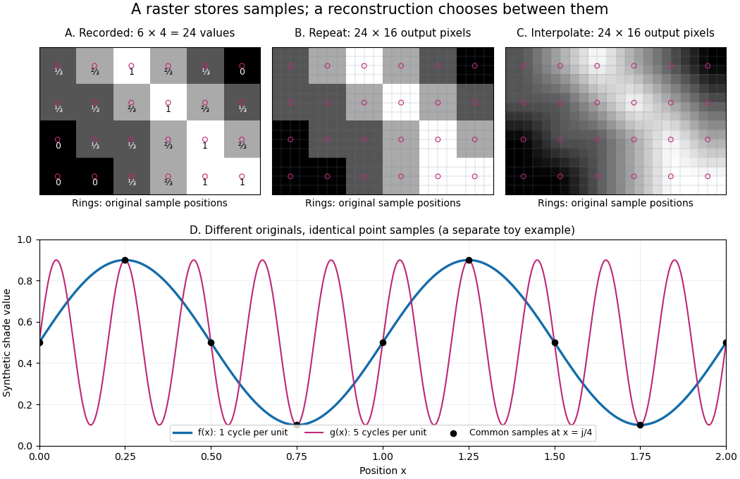
The upper panels start with exactly the same array. Nearest-neighbor interpolation repeats its values into a display; successive linear interpolations in the two coordinate directions produce a smoother display. Original sample positions are marked. Both displays use 384 output pixels, but only the same 24 recorded values. The extra values follow the chosen interpolation rule. Between-grid appearance is inferred, not independently recorded.
Spatial resolution needs a stated meaning. A grid over a rectangle of width and height has nominal cell pitches and . Over the same rectangle, doubling both dimensions halves these pitches and quadruples the pixel count. That is a finer grid, not a guarantee of more recoverable detail. Blurring before sampling, quantization and aliasing can make different originals share the same recorded array. Enlarging the rectangle without adding samples instead increases the displayed pitch.
A reproducible computational demonstration makes the ambiguity exact. Take the one-dimensional profiles and , repeated identically along every row. Sample at for . Since , the fact that the sine is a periodic function gives . Both yield , although at they give approximately and . The lower panel draws both originals and their common samples: no operation on those samples alone can identify the original profile. This is aliasing in an ideal point-sampling model, without image noise or rounding.
The Nyquist–Shannon sampling theorem describes reconstruction under a bandwidth restriction and ideal sampling assumptions; it does not grant uniqueness for arbitrary image signals from a finite raster image.[ref]
https://fab.cba.mit.edu/classes/S62.12/docs/Shannon_noise.pdf. Shannon, Communication in the Presence of Noise (1949), section II, Theorem 1 and reconstruction from the infinite sample sequence
The beautiful lesson is constructive: choose what detail the grid should preserve before sampling, and choose a reconstruction rule suited to the information actually retained.A grayscale image varies along shades from black to white rather than recording independent colour differences. A numerical grayscale image assigns one shade sample to each pixel; an encoding determines how that sample maps to a displayed shade. A colour raster image can also look grayscale, for example when its three sRGB components are equal.
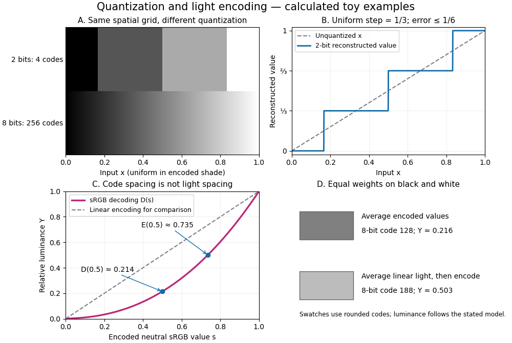


The convention in our lossy block averaging example is black at the integer code 0 and white at 255. Its arithmetic means act on those stored codes. This is a fully specified numerical experiment, but it does not claim that code 128 means half the physical light of code 255. PNG explicitly allows samples that are not proportional to light: its grayscale interpretation depends on the indicated transfer curve, and can be device-dependent when that information is absent.[ref]
https://www.w3.org/TR/png-3/#6Colour-values. W3C, PNG Specification, Third Edition, section 6.1: colour types, grayscale interpretation and transfer curves
Two different questions therefore need different operations. To average stored codes, average the integers. To average relative luminance for neutral sRGB shades, decode the codes to linear light, average there, and encode the result again. Equal weights on black and white give encoded value by the first method, but approximately by the second. Rounded to eight-bit codes these are 128 and 188. This example concerns ideal neutral shades and the specified sRGB conversion; it does not assert a universal grayscale conversion for every colour encoding.
The upper panels hold the spatial grid fixed and change sample depth: four levels produce broad constant bands, while 256 levels make smaller numerical steps. The lower panels hold the colour interpretation fixed and compare encoded sRGB values with relative luminance. All panels are calculated synthetic examples, not measured display data. Grayscale is useful when shade structure is the quantity of interest: a synthetic scalar image signal can be inspected without introducing separate colour components.
A pixel is one picture element at an indexed position in a raster image. It can contain a single grayscale value or several colour components. The word can also refer to a physical display element; the indexed element of the stored image is the meaning used here. One stored pixel need not occupy exactly one physical display element when the image is resized. Microsoft's bitmap documentation likewise distinguishes an image's grid and its numerical colour representation.[ref]
https://learn.microsoft.com/en-us/windows/win32/gdi/about-bitmaps. Microsoft Learn, About Bitmaps: pixel grids and bitmap representations
Separate position from value: raster sampling and reconstruction concerns the spatial grid, while sample depth concerns how many bits encode each component. Four times as many pixels can describe a finer grid without improving the quantization of any value. Conversely, more bits per sample can distinguish more shades without locating an edge more precisely.
Light initiates methane chlorination by photodissociation of through homolysis. The elementary bookkeeping isHere denotes the photon energy. The first propagation step replaces a chlorine radical with a methyl radical; the second regenerates a chlorine radical. Adding the two propagation equations cancels both free radicals and gives : chloromethane and hydrogen chloride are made while the chain carrier is regenerated.[ref]
6.6 Radical Reactions. Organic Chemistry by John McMurry, §6.6: chlorine photolysis and the two-step methane chlorination cycle
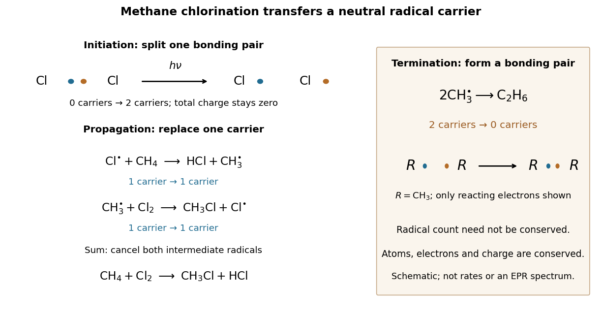
Methane chlorination: initiation supplies carriers, propagation replaces them, termination removes them
. The left panel follows the reacting electron pair in homolysis, then counts chain carriers through two propagation steps. The right panel shows recombination termination. Every chemical species in this example is neutral. Electron marks are bookkeeping, not a measured electronic wavefunction or a reaction-rate plot. Details.
For example, recombination of methyl radicals makes ethane and a covalent bond from two unpaired electrons, removing two carriers. Recombination of two also terminates carriers; in the gas phase, stabilization of the product requires disposal of released energy, for example to a third collision partner. The figure omits that partner. Termination competes with propagation, and further chlorination can consume chloromethane, so this cycle alone does not predict a pure product or a measured reaction rate.[ref]
10.2 Preparing Alkyl Halides from Alkanes: Radical Halogenation. Organic Chemistry by John McMurry, §10.2, Figure 10.2 and following paragraphs: radical combination terminates the chain; further substitution gives product mixtures
There are unlisted articles, also show them or only show them.