
Prey is an organism consumed by a predator in predation. The name describes the receiving end of that interaction: a small fish can be prey for a large fish while being a predator of zooplankton. In a food web drawn with resource-to-consumer arrows, a feeding arrow goes outward from the prey toward its predator. This convention makes the route of food and energy easy to follow.
Linkage disequilibrium means that knowing an allele at one genetic locus changes the probability of an allele at another genetic locus in population haplotypes. It compares their joint probability distribution with the product of their marginal distributions. This is useful because a genetic marker can carry information about another genetic locus: tag SNPs exploit this redundancy, without establishing a causal genetic association.
Consider two genetic loci with alleles and . Sample one haplotype, rather than an unphased diploid genotype. Write its four haplotype frequencies as , summing to one, and set the marginal allele frequencies to and . The linkage disequilibrium coefficient isThe second expression follows by substituting . The entire two-locus joint probability distribution is thenEvery row and column sum is unchanged when varies. Linkage equilibrium means : all four haplotype frequencies equal products of allele frequencies, so the two allele indicators are independent random variables. For , the conditional probability shows directly how positive enriches among copies carrying , while negative depletes it. Positive also enriches ; negative enriches and . Swapping the labels and reverses the sign of , so neither sign is intrinsically favorable.
For example, fix the allele frequencies at . At linkage equilibrium, the haplotype frequencies in the order are . Positive linkage disequilibrium instead gives , with ; negative linkage disequilibrium gives , with . Counting each allele separately would miss the difference.
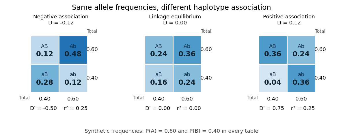
Three haplotype joint probability distributions with identical marginal allele frequencies, showing negative linkage disequilibrium, linkage equilibrium and positive linkage disequilibrium
. Details. 
Nonnegative haplotype frequencies constrain . Define the nonnegative bounds and . The four entries above giveThus globally, but a particular pair of allele frequencies usually permits a smaller, asymmetric interval. The standardized linkage disequilibrium convention used here retains the sign:This convention requires ; if either genetic locus has only one allele in the population, but normalized measures are undefined. Some presentations report only . At or , at least one of the four haplotypes has zero frequency; this alone does not prove that genetic recombination has never occurred.
For the indicator random variables and , their covariance is , and their variances are and . The allelic correlation measure is their squared correlation coefficient,The subscript distinguishes it from the recombination fraction in linkage-disequilibrium decay under recombination. Squaring loses the association's sign. In the illustrated positive and negative examples, in both, whereas and , respectively. For another original example, take : then , yet . Every carries , but most copies carrying lack . The frequency constraints and the distinction between these normalizations are analyzed in Mathematical properties of the r² measure of linkage disequilibrium by Jenna M. VanLiere and others (sections 2.1 and 2.5, pp. 131–132 and 135–136).
Genetic linkage describes transmission through meiosis; linkage disequilibrium describes a population's haplotype frequencies. Nearby genetic loci on a chromosome can be in linkage equilibrium. Conversely, mixing populations can create linkage disequilibrium even between genetic loci on different chromosomes. For example, mix equal numbers of independently sampled haplotypes from two populations, each internally at linkage equilibrium, with in one and in the other. The pooled allele frequencies are , but , giving . This is a consequence of population stratification, not a measurement of the recombination fraction.
Measured haplotype frequencies also depend on the sample. Finite sample size, related individuals, genetic-study ascertainment, genotyping error and uncertain haplotype estimation can change an estimate. A missing rare haplotype can give empirical without demonstrating its absence from the population. Report the sample definition and allele frequencies alongside the association measure; a nonzero sample estimate alone does not establish nonzero population linkage disequilibrium.
A concrete dataset is the 2005 A haplotype map of the human genome by The International HapMap Consortium. The International HapMap Consortium used genotyping platforms including Illumina BeadArray to obtain SNP genotype calls from 269 DNA samples across four collections: 30 parent–offspring trios from Ibadan, 30 trios from Utah, 45 unrelated individuals from Beijing and 44 from Tokyo. Parent–offspring trios and the PHASE algorithm supplied haplotype estimation, rather than direct observation of every chromosome. In Figure 7, 36 SNPs resolve seven haplotypes in a chromosome 2 region in the Utah panel; seven tag SNPs capture the 36 SNPs at . The readout demonstrates reusable allelic correlation, not causal effects.
Controls required over 80% complete calls, at most one discordance among five duplicate genotypes, at most one Mendelian segregation error per trio panel, and a Hardy-Weinberg equilibrium test with ; blind reassessment checked performance. Minor allele frequencies of at least 0.05 were targeted, the collections were not population-representative, and inferred haplotypes retain phase uncertainty. These limits restrict extrapolation of linkage disequilibrium.[ref]
A haplotype map of the human genome by The International HapMap Consortium. pp. 1300–1302, Table 1; Figure 7, p. 1306; Methods, p. 1316
Inbreeding is reproduction between genetically related individuals. It increases the chance that an offspring's maternal and paternal copies at a locus are identical by descent. Such homozygosity by descent is autozygosity.
The infinite-sites model assumes that every mutation occurs at a previously unmutated site, so each mutation on the sample genealogy produces a distinct segregating site. If mutation rate per lineage is in standard coalescent time units, a tree of total length has a Poisson distribution of mutation count with mean .
A segregating site is a position at which at least two states occur in the sampled chromosomes. Under an infinite sites mutation model, mutations below the sample's common ancestor correspond one-to-one to segregating sites. Their number is commonly denoted .
Effective population size is the size of an idealized biological population giving the relevant rate of genetic drift or ancestral coalescence in the biological population being modeled. In the standard neutral diploid coalescent, time is measured in generations and the population-scaled mutation parameter is .
// Target: biology.bigb
Genetic drift is random variation of allele frequencies due to finite-population reproduction. In the neutral ancestry description, randomly sampled gene copies merge into common ancestors according to Kingman's coalescent.
// Target: probability-and-statistics.bigb
A population bottleneck is a temporary large decrease in biological population size. It changes ancestral coalescence rates and can leave fewer ancestral haplotypes and increased linkage disequilibrium after the biological population expands.
// Target: biology.bigb
An ancestral recombination graph records ancestral coalescences and genetic recombination events for sampled chromosomal material. Backwards in time, each pair of ancestral lineages merges at rate one in standard diploid coalescent units, while a lineage splits at a recombination breakpoint at rate times the genetic span of the material it carries. The breakpoint splits that lineage's ancestral material into two parental contributions. Waiting times are exponential with the sum of the current event rates. At each genomic position, retaining the ancestry at that position gives a marginal phylogenetic tree with the neutral Kingman's coalescent distribution. Different positions have dependent trees because they share parts of the graph.
// Target: biology.bigb
Genotype fitness measures the reproductive or viability success assigned to a genotype in a specified selection model. Relative fitnesses weight Hardy-Weinberg proportions after viability selection; continuous-time fitness differences instead act as selection-rate differences. The convention and time units must be specified before comparing selection with migration.
Underdominance means that the heterozygote has lower genotype fitness than both corresponding homozygotes. In a deterministic randomly mating biallelic biological population, it produces an unstable interior allele-frequency threshold separating the two fixation outcomes, unlike heterozygote advantage.
A heterozygote has greater genotype fitness than either corresponding homozygote. In the deterministic random-mating two-allele viability-selection model this gives an attracting interior allele frequency, unlike the repelling interior frequency produced by underdominance.
The protein backbone is the repeating chain of chemical atoms that connects successive amino acid residues, including their peptide bonds. The attached groups that distinguish amino acids project from this shared framework. Protein folding changes the framework's spatial arrangement while ordinarily preserving its sequence connectivity. See Cooper: polypeptide backbone and attached groups.
A peptide bond is the covalent bond between the carboxyl carbon of one amino acid residue and the amino nitrogen of the next. The displayed group shows the usual linkage, with the central carbon–nitrogen connection being the peptide bond. In an intact unbranched chain of amino acid residues, adjacent positions supply peptide bonds. Cutting one internal peptide bond produces two fragments; merely changing the chain's shape need not cut it. See Clark, Douglas and Choi, Biology 2e: peptide bonds and protein structure.
An amino acid residue is the portion of an amino acid incorporated into a polypeptide chain. For example, the A in the illustrative protein primary structure is an alanine residue, rather than a free alanine molecule floating beside the chain. Counting amino acid residues counts chain positions; repeated letters are separate positions. See IUPAC-IUB, section 3AA-16: symbols for amino-acid residues.
In chain-growth polymerization, each growth step joins a monomer to a reactive site on a polymer chain and regenerates that reactive site. This is the precise mechanistic restriction in IUPAC's definition: growth occurs exclusively through these monomer–chain-site reactions. The word chain refers to the succession of site-regenerating chemical reactions. It does not merely mean that the product looks like a long chain. Chain-growth initiation starts this succession; chain-growth propagation continues it; chain-growth termination and chain transfer in chain polymerization can change its fate.[ref]
IUPAC Compendium of Chemical Terminology, fifth edition (Gold Book) by International Union of Pure and Applied Chemistry. chain polymerization, C00958, definition and notes 1–2; source recommendation p. 2306
The contrast with step-growth polymerization concerns the permitted joining partners. There, suitable reactive groups can join two existing chains, for example a two-unit chain and a three-unit chain. In chain-growth propagation, a free monomer adds to a polymerization-active site. Release of a small byproduct is a separate classification question: IUPAC explicitly allows condensative chain polymerization.[ref]
IUPAC Compendium of Chemical Terminology, fifth edition (Gold Book) by International Union of Pure and Applied Chemistry. chain polymerization, C00958, notes 3–6
The useful consequence is that a few growing chains can incorporate many monomer molecules while much of the feed remains unreacted. Their degree of polymerization depends on how those units are shared among chains, as finite chain-growth bookkeeping makes explicit.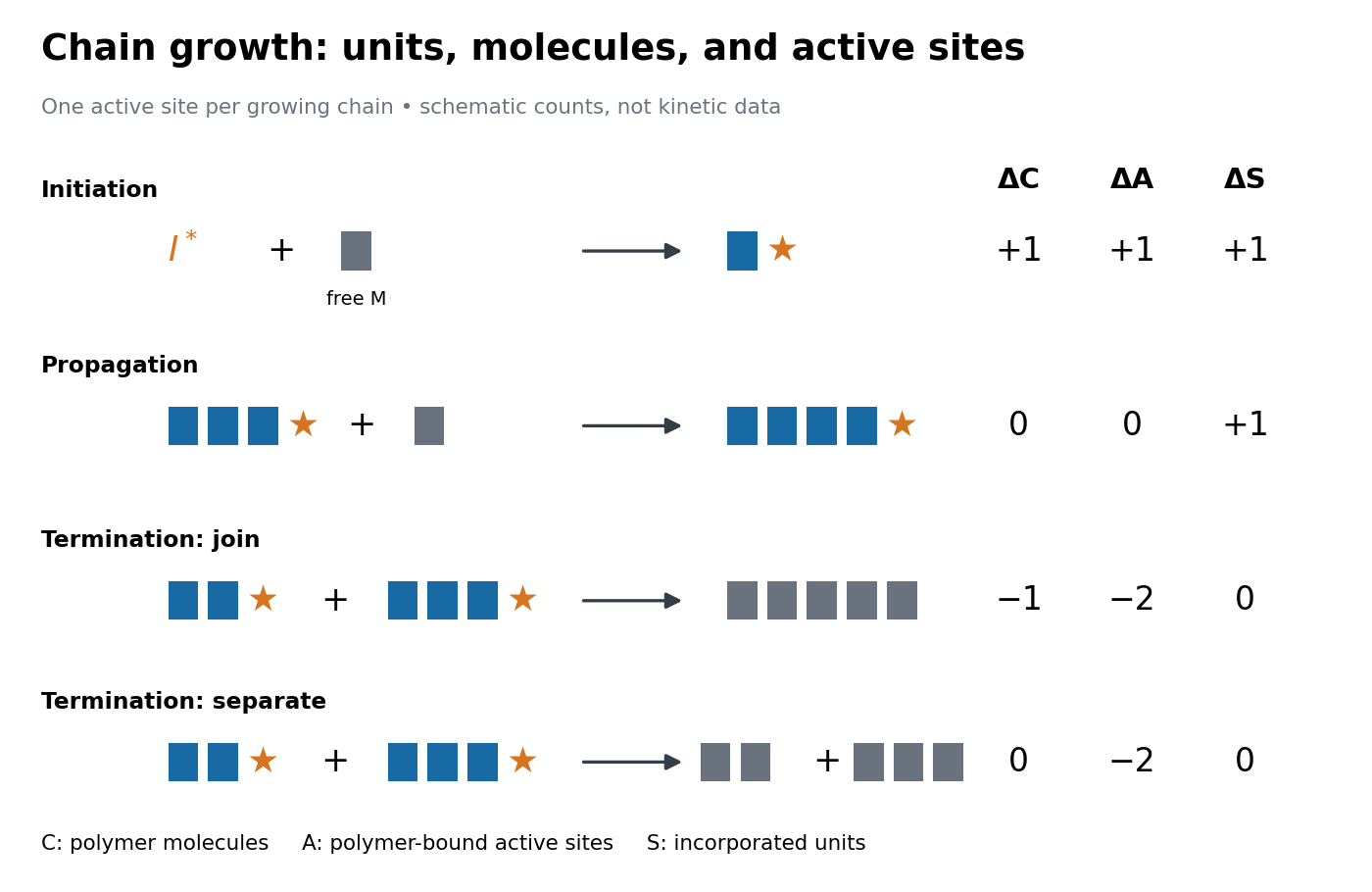

Gelation is formation of an extended connected network. In step-growth polymerization, feed molecules with functionality in polymerization above two can introduce branching and permit gelation. The linear step-growth molecule count's two-ended-chain interpretation and bifunctional Carothers equation must not silently be applied to such networks. Each join between distinct connected pieces still reduces their count by one, but neither that identity nor average size alone specifies the onset of gelation.
The functionality in polymerization is the number of reactive functional groups on a molecule for the specified joining chemistry. The linear step-growth molecule count assumes for every feed molecule. A diol supplies two hydroxy groups in the polyurethane example; an impurity supplying only one suitable group can cap a chain. A group count must reflect the selected chemical reaction, not simply every chemically recognizable group in the molecule.
In step-growth polymerization, suitable reactive groups on molecules of different chain lengths can join. The linear count and its assumptions are given in polymerization.
A one-unit monomer, a two-unit chain, and a twenty-unit chain can all be joining partners if their functional groups are compatible and accessible. Schematically, : the subscripts count monomeric units, and end-group chemistry is suppressed. In chain-growth propagation, by contrast, requires a free monomer and a polymerization-active site. An arbitrary pair of existing chains is not a propagation pair in that mechanism. The practical consequence of step-growth polymerization is that most monomers can have joined something while the average chain is still short.
Whether a joining step releases a small molecule is a separate question. Polycondensation releases small products during the joining chemistry, as in the Nylon 6,10 demonstration in polymerization. Polyaddition joins suitable chains without that elimination: reacting a diol with a molecule bearing two isocyanate groups can build a polyurethane. Thus step-growth polymerization and polycondensation are not synonyms.[ref]
IUPAC Compendium of Chemical Terminology, fifth edition (Gold Book) by International Union of Pure and Applied Chemistry. polyaddition, P04720, definition and note 1; polycondensation, P04722, definition and growth-step equation; source recommendation p. 2307
Unpolarized light has no preferred transverse polarization direction in its time-averaged statistics. An ideal linear polarizer transmits half its incident light intensity: equal transverse components give the averaged projection factor . This statistical description differs from the fixed deterministic phase relation of a monochromatic wave in a pure polarization of waves state.
There are unlisted articles, also show them or only show them.